Set-up

SESOI

Measures

Well-being
Social media use
Social media channels
Locus of control
Table
Figure

Analyses

Multicollinearity
Correlations
Publication
Standardized results
Figures
Table

Save workspace

Here you can find the code and the results of all main analyses.
To see the code, click on button “Code”.
Alternatively, you can download the rmd file from the github repo.

Set-up

Load packages & workspace.

# install packages
## devtools::install_github("https://github.com/tdienlin/td@v.0.0.2.5")

# define packages
library(broom.mixed)
library(brms)
library(corrr)
library(devtools)
library(GGally)
library(ggplot2)
library(gridExtra)
library(kableExtra)
library(knitr)
library(lavaan)
library(lme4)
library(magrittr)
library(mice)
library(PerFit)
library(performance)
library(psych)
library(quanteda.textstats)
library(scales)
library(semTools)
library(tidyverse)
library(td)

# load workspace
load("data/workspace_1.RData")

SESOI

In what follows, more information on how the SESOI was defined exactly.

If people can reliably differentiate 7 levels, this corresponds to 11 / 7 = 1.57 unit change on an 11-point scale. Hence, a four-point change in media use (e.g., a complete stop) should result in a 1.57-point change in life satisfaction. In a statistical regression analysis, b estimates the change in the dependent variable if the independent variable increases by one point. For life satisfaction, we would therefore define a SESOI of b = 1.57 / 4 = 0.39. For positive or negative affect, which was measured on a 5-point scale, our SESOI would be b = 0.71 / 4 = 0.18. Because we are agnostic as to whether the effects are positive or negative, the null region includes both negative and positive effects. Finally, in order not to exaggerate precision and to be less conservative, these numbers are reduced to nearby thresholds. Note that other researchers also decreased or recommended decreasing thresholds for effect sizes when analyzing within-person or cumulative effects (Beyens et al. 2021; Funder and Ozer 2019).

Measures

Let’s first inspect the individual measures, how they develop over time. For positive and negative affect, we also look at their factor structure, as they’re measured with multiple items.

Well-being

Life satisfaction

Let’s inspect the development of life satisfaction across the study. We nest reponses inside participants and waves to get better results.

fit_life_sat <- lmer(life_sat ~ (1 | id) + (1 | wave), d_long_100_imp)
summary(fit_life_sat)

## Linear mixed model fit by REML ['lmerMod']
## Formula: life_sat ~ (1 | id) + (1 | wave)
##    Data: d_long_100_imp
## 
## REML criterion at convergence: 558297
## 
## Scaled residuals: 
##    Min     1Q Median     3Q    Max 
## -4.021 -0.504  0.164  0.648  3.900 
## 
## Random effects:
##  Groups   Name        Variance Std.Dev.
##  id       (Intercept) 1.11455  1.0557  
##  wave     (Intercept) 0.00534  0.0731  
##  Residual             4.99443  2.2348  
## Number of obs: 123794, groups:  id, 3639; wave, 34
## 
## Fixed effects:
##             Estimate Std. Error t value
## (Intercept)   6.4900     0.0224     289

dat_fig_life_sat <- data.frame(type = "Life satisfaction", dimension = "Life satisfaction", 
                               get_dat(fit_life_sat))
make_graph(dat_fig_life_sat, "Life Satisfaction", 1, 10)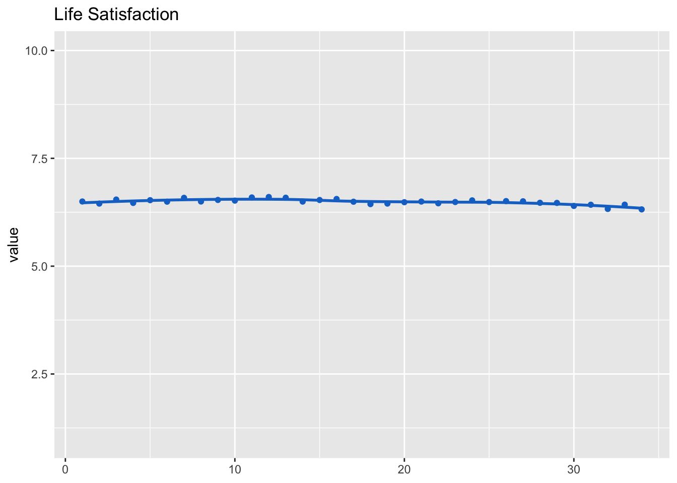

Positive affect

Let’s next expect the development across waves.

model_aff_pos <- lmer(aff_pos_m ~ (1 | id) + (1 | wave), d_long_100_imp)
summary(model_aff_pos)

## Linear mixed model fit by REML ['lmerMod']
## Formula: aff_pos_m ~ (1 | id) + (1 | wave)
##    Data: d_long_100_imp
## 
## REML criterion at convergence: 344960
## 
## Scaled residuals: 
##    Min     1Q Median     3Q    Max 
## -3.890 -0.699 -0.010  0.701  3.847 
## 
## Random effects:
##  Groups   Name        Variance Std.Dev.
##  id       (Intercept) 0.27487  0.5243  
##  wave     (Intercept) 0.00142  0.0377  
##  Residual             0.88348  0.9399  
## Number of obs: 123794, groups:  id, 3639; wave, 34
## 
## Fixed effects:
##             Estimate Std. Error t value
## (Intercept)   3.1570     0.0112     283

dat_fig_aff_pos <- data.frame(type = "Affect", dimension = "Positive", 
                              get_dat(model_aff_pos))
make_graph(dat_fig_aff_pos, "Positive Affect", 1, 5)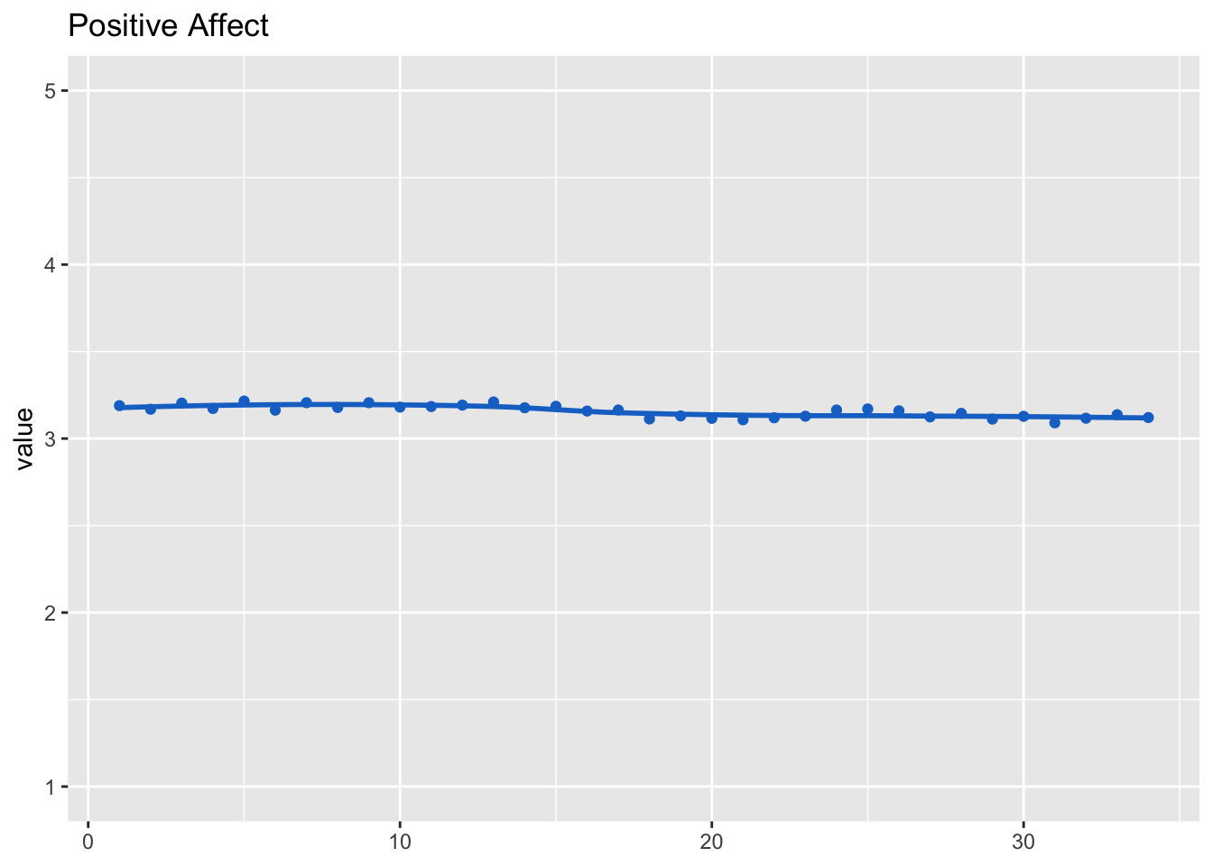

Positive affect was measured as a scale. We hence also inspect factorial validity using CFA.

We first test assumption of multivariate normality. We focus on wave 1 here.

d_long_100_imp %>%
  filter(wave == 1) %>%
  select(aff_pos_1, aff_pos_2, aff_pos_3) %>% 
  mardia()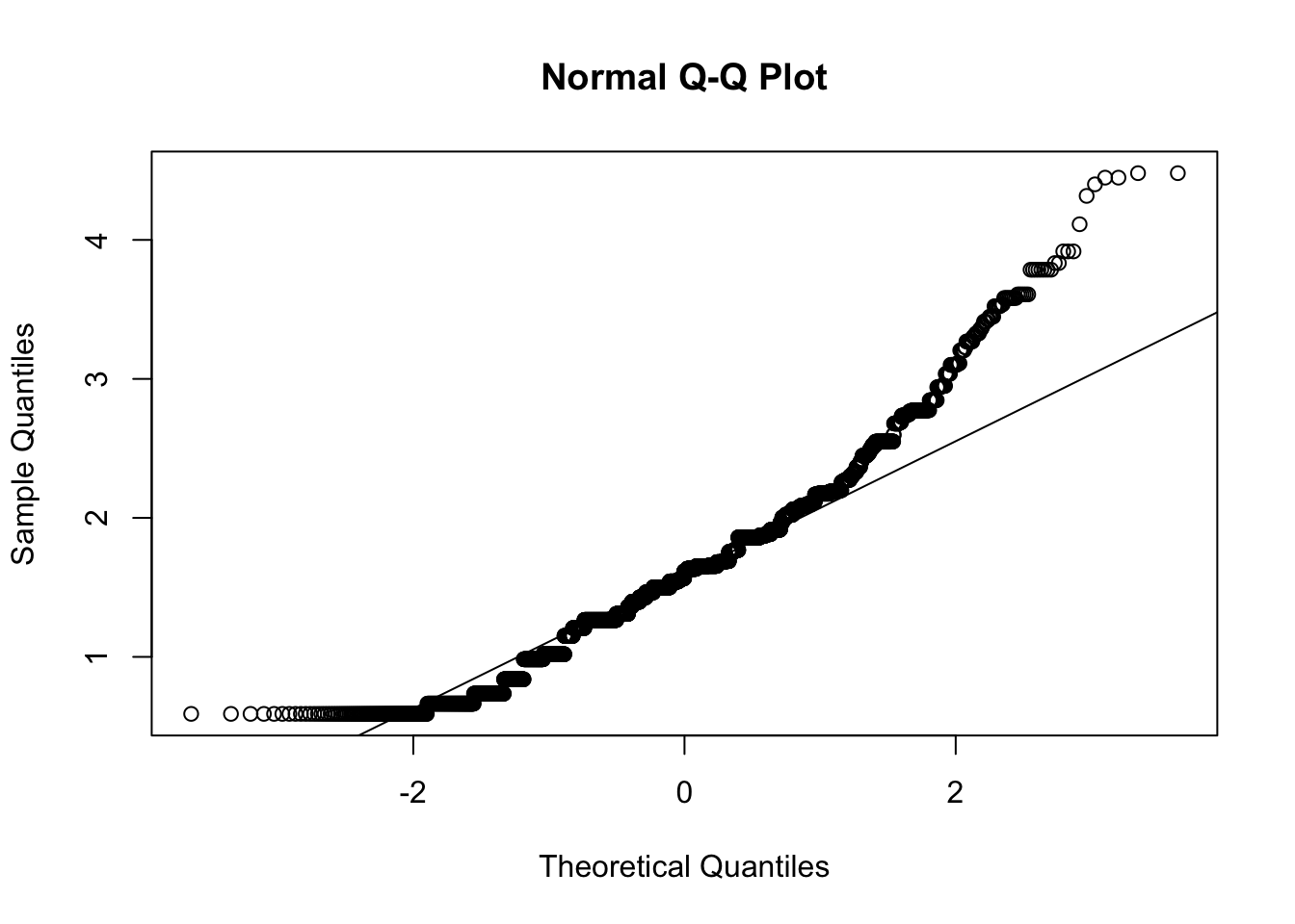

## Call: mardia(x = .)
## 
## Mardia tests of multivariate skew and kurtosis
## Use describe(x) the to get univariate tests
## n.obs = 3641   num.vars =  3 
## b1p =  0.33   skew =  202  with probability  <=  0.000000000000000000000000000000000000067
##  small sample skew =  202  with probability <=  0.000000000000000000000000000000000000059
## b2p =  14   kurtosis =  -3  with probability <=  0.0026

Assumption of multivariate normal distribution was violated; hence, robust estimator will be used.

model <- "
aff_pos =~ a1*aff_pos_1 + a2*aff_pos_2 + a3*aff_pos_3
"
cfa_aff_pos <- cfa(model, d_long_100_imp, group = "wave", estimator = "MLM")
summary(cfa_aff_pos, standardized = TRUE, fit = TRUE, estimates = FALSE)

## lavaan 0.6.15 ended normally after 105 iterations
## 
##   Estimator                                         ML
##   Optimization method                           NLMINB
##   Number of model parameters                       306
##   Number of equality constraints                    66
## 
##   Number of observations per group:                   
##     1                                             3641
##     2                                             3641
##     3                                             3641
##     4                                             3641
##     5                                             3641
##     6                                             3641
##     7                                             3641
##     8                                             3641
##     9                                             3641
##     10                                            3641
##     11                                            3641
##     12                                            3641
##     13                                            3641
##     14                                            3641
##     15                                            3641
##     16                                            3641
##     17                                            3641
##     18                                            3641
##     19                                            3641
##     20                                            3641
##     21                                            3641
##     22                                            3641
##     23                                            3641
##     24                                            3641
##     25                                            3641
##     26                                            3641
##     27                                            3641
##     28                                            3641
##     29                                            3641
##     30                                            3641
##     31                                            3641
##     32                                            3641
##     33                                            3641
##     34                                            3641
## 
## Model Test User Model:
##                                               Standard      Scaled
##   Test Statistic                                91.607     101.525
##   Degrees of freedom                                66          66
##   P-value (Chi-square)                           0.020       0.003
##   Scaling correction factor                                  0.902
##     Satorra-Bentler correction                                    
##   Test statistic for each group:
##     1                                            6.200       6.872
##     2                                            5.536       6.136
##     3                                            5.844       6.476
##     4                                            1.182       1.310
##     5                                            0.243       0.270
##     6                                            0.006       0.007
##     7                                            7.124       7.895
##     8                                            6.115       6.778
##     9                                            1.938       2.148
##     10                                           0.211       0.234
##     11                                           2.453       2.718
##     12                                           0.855       0.948
##     13                                           1.621       1.796
##     14                                           2.235       2.477
##     15                                           1.416       1.569
##     16                                           0.859       0.952
##     17                                           2.557       2.834
##     18                                           1.181       1.308
##     19                                          10.398      11.524
##     20                                           1.344       1.489
##     21                                           3.255       3.608
##     22                                           3.063       3.394
##     23                                           1.986       2.201
##     24                                           0.896       0.993
##     25                                           1.131       1.254
##     26                                           0.212       0.235
##     27                                           1.368       1.516
##     28                                           6.273       6.952
##     29                                           0.975       1.080
##     30                                           3.190       3.535
##     31                                           1.845       2.044
##     32                                           0.580       0.643
##     33                                           6.614       7.330
##     34                                           0.902       0.999
## 
## Model Test Baseline Model:
## 
##   Test statistic                            162556.114  182172.729
##   Degrees of freedom                               102         102
##   P-value                                        0.000       0.000
##   Scaling correction factor                                  0.892
## 
## User Model versus Baseline Model:
## 
##   Comparative Fit Index (CFI)                    1.000       1.000
##   Tucker-Lewis Index (TLI)                       1.000       1.000
##                                                                   
##   Robust Comparative Fit Index (CFI)                         1.000
##   Robust Tucker-Lewis Index (TLI)                            1.000
## 
## Loglikelihood and Information Criteria:
## 
##   Loglikelihood user model (H0)            -521289.317 -521289.317
##   Loglikelihood unrestricted model (H1)    -521243.514 -521243.514
##                                                                   
##   Akaike (AIC)                             1043058.634 1043058.634
##   Bayesian (BIC)                           1045392.964 1045392.964
##   Sample-size adjusted Bayesian (SABIC)    1044630.235 1044630.235
## 
## Root Mean Square Error of Approximation:
## 
##   RMSEA                                          0.010       0.012
##   90 Percent confidence interval - lower         0.004       0.007
##   90 Percent confidence interval - upper         0.015       0.017
##   P-value H_0: RMSEA <= 0.050                    1.000       1.000
##   P-value H_0: RMSEA >= 0.080                    0.000       0.000
##                                                                   
##   Robust RMSEA                                               0.012
##   90 Percent confidence interval - lower                     0.007
##   90 Percent confidence interval - upper                     0.016
##   P-value H_0: Robust RMSEA <= 0.050                         1.000
##   P-value H_0: Robust RMSEA >= 0.080                         0.000
## 
## Standardized Root Mean Square Residual:
## 
##   SRMR                                           0.008       0.008

The data fit the model very well, $\chi^2$ (66) = 91.61, p = .020, CFI = 1.00, RMSEA = .01, 90% CI [< .01, .02], SRMR < .01. Let’s next inspect reliability.

rel_aff_pos <- get_rel(cfa_aff_pos)

The average reliability across all waves was omega = 0.85, hence good.

Let’s now export factor scores for results reported in additional analyses.

# with imputed data
cfa_aff_pos_50 <- cfa(model, d_long_50_imp, group = "wave", estimator = "MLM")
d_long_50_imp$aff_pos_fs <- get_fs(cfa_aff_pos_50)

# without imputed data
cfa_aff_pos <- cfa(model, d_long_50, group = "wave", estimator = "MLM")
d_long_50$aff_pos_fs <- get_fs(cfa_aff_pos)

Negative affect

model_aff_neg <- lmer(aff_neg_m ~ (1 | id) + (1 | wave), d_long_100_imp)
summary(model_aff_neg)

## Linear mixed model fit by REML ['lmerMod']
## Formula: aff_neg_m ~ (1 | id) + (1 | wave)
##    Data: d_long_100_imp
## 
## REML criterion at convergence: 294736
## 
## Scaled residuals: 
##    Min     1Q Median     3Q    Max 
## -4.313 -0.572 -0.192  0.295  4.841 
## 
## Random effects:
##  Groups   Name        Variance Std.Dev.
##  id       (Intercept) 0.20084  0.4482  
##  wave     (Intercept) 0.00123  0.0351  
##  Residual             0.58731  0.7664  
## Number of obs: 123794, groups:  id, 3639; wave, 34
## 
## Fixed effects:
##             Estimate Std. Error t value
## (Intercept)  1.80813    0.00981     184

dat_fig_aff_neg <- data.frame(type = "Affect", dimension = "Negative", get_dat(model_aff_neg))
make_graph(dat_fig_aff_neg, "Negative Affect", 1, 5)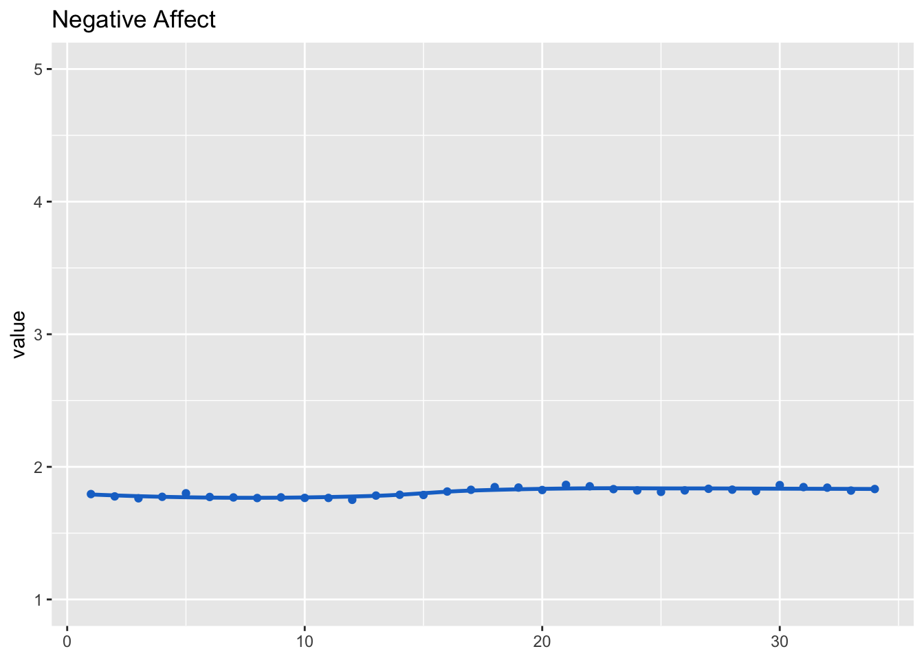

Negative affect was measured as a scale. We hence inspect factorial validity using CFA.

We first test assumption of multivariate normality. We’ll focus on wave 1 here.

d_long_100_imp %>%
  filter(wave == 1) %>% 
  select(aff_neg_1, aff_neg_2, aff_neg_3, aff_neg_4, aff_neg_5, aff_neg_6) %>% 
  mardia()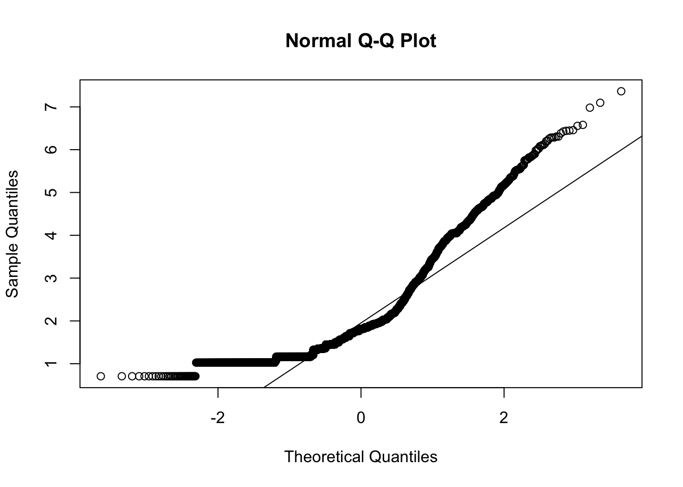

## Call: mardia(x = .)
## 
## Mardia tests of multivariate skew and kurtosis
## Use describe(x) the to get univariate tests
## n.obs = 3641   num.vars =  6 
## b1p =  13   skew =  7773  with probability  <=  0
##  small sample skew =  7782  with probability <=  0
## b2p =  85   kurtosis =  114  with probability <=  0

Assumption of multivariate normal distribution was violated; hence, robust estimator will be used.

model <- "
aff_neg =~ a1*aff_neg_1 + a2*aff_neg_2 + a3*aff_neg_3 + a4*aff_neg_4 + a5*aff_neg_5 + a6*aff_neg_6
"
cfa_aff_neg <- cfa(model, d_long_100_imp, group = "wave", estimator = "MLM")
summary(cfa_aff_neg, standardized = TRUE, fit = TRUE, estimates = FALSE)

## lavaan 0.6.15 ended normally after 105 iterations
## 
##   Estimator                                         ML
##   Optimization method                           NLMINB
##   Number of model parameters                       612
##   Number of equality constraints                   165
## 
##   Number of observations per group:                   
##     1                                             3641
##     2                                             3641
##     3                                             3641
##     4                                             3641
##     5                                             3641
##     6                                             3641
##     7                                             3641
##     8                                             3641
##     9                                             3641
##     10                                            3641
##     11                                            3641
##     12                                            3641
##     13                                            3641
##     14                                            3641
##     15                                            3641
##     16                                            3641
##     17                                            3641
##     18                                            3641
##     19                                            3641
##     20                                            3641
##     21                                            3641
##     22                                            3641
##     23                                            3641
##     24                                            3641
##     25                                            3641
##     26                                            3641
##     27                                            3641
##     28                                            3641
##     29                                            3641
##     30                                            3641
##     31                                            3641
##     32                                            3641
##     33                                            3641
##     34                                            3641
## 
## Model Test User Model:
##                                               Standard      Scaled
##   Test Statistic                              8941.917    5116.110
##   Degrees of freedom                               471         471
##   P-value (Chi-square)                           0.000       0.000
##   Scaling correction factor                                  1.748
##     Satorra-Bentler correction                                    
##   Test statistic for each group:
##     1                                          376.324     215.313
##     2                                          413.969     236.852
##     3                                          328.789     188.116
##     4                                          276.199     158.027
##     5                                          303.113     173.426
##     6                                          272.462     155.889
##     7                                          251.993     144.178
##     8                                          219.985     125.864
##     9                                          284.157     162.580
##     10                                         254.619     145.680
##     11                                         293.673     168.024
##     12                                         293.655     168.014
##     13                                         243.299     139.203
##     14                                         218.850     125.215
##     15                                         192.210     109.973
##     16                                         260.088     148.809
##     17                                         292.880     167.571
##     18                                         237.822     136.070
##     19                                         200.681     114.820
##     20                                         180.729     103.404
##     21                                         204.462     116.983
##     22                                         238.017     136.181
##     23                                         288.489     165.059
##     24                                         221.483     126.721
##     25                                         321.760     184.095
##     26                                         212.502     121.583
##     27                                         216.358     123.789
##     28                                         273.754     156.628
##     29                                         238.662     136.551
##     30                                         237.627     135.958
##     31                                         282.783     161.794
##     32                                         289.459     165.614
##     33                                         188.099     107.621
##     34                                         332.965     190.506
## 
## Model Test Baseline Model:
## 
##   Test statistic                            475665.865  176291.139
##   Degrees of freedom                               510         510
##   P-value                                        0.000       0.000
##   Scaling correction factor                                  2.698
## 
## User Model versus Baseline Model:
## 
##   Comparative Fit Index (CFI)                    0.982       0.974
##   Tucker-Lewis Index (TLI)                       0.981       0.971
##                                                                   
##   Robust Comparative Fit Index (CFI)                         0.983
##   Robust Tucker-Lewis Index (TLI)                            0.981
## 
## Loglikelihood and Information Criteria:
## 
##   Loglikelihood user model (H0)            -868181.412 -868181.412
##   Loglikelihood unrestricted model (H1)    -863710.454 -863710.454
##                                                                   
##   Akaike (AIC)                             1737256.824 1737256.824
##   Bayesian (BIC)                           1741604.513 1741604.513
##   Sample-size adjusted Bayesian (SABIC)    1740183.930 1740183.930
## 
## Root Mean Square Error of Approximation:
## 
##   RMSEA                                          0.070       0.052
##   90 Percent confidence interval - lower         0.069       0.051
##   90 Percent confidence interval - upper         0.072       0.053
##   P-value H_0: RMSEA <= 0.050                    0.000       0.000
##   P-value H_0: RMSEA >= 0.080                    0.000       0.000
##                                                                   
##   Robust RMSEA                                               0.069
##   90 Percent confidence interval - lower                     0.067
##   90 Percent confidence interval - upper                     0.071
##   P-value H_0: Robust RMSEA <= 0.050                         0.000
##   P-value H_0: Robust RMSEA >= 0.080                         0.000
## 
## Standardized Root Mean Square Residual:
## 
##   SRMR                                           0.021       0.021

The data fit the model very well, $\chi^2$ (471) = 8941.92, p < .001, CFI = .98, RMSEA = .07, 90% CI [.07, .07], SRMR = .02.

Let’s next inspect reliability.

rel_aff_neg <- get_rel(cfa_aff_neg)

The average reliability across all waves was omega = 0.91, hence good.

model_aff_neg <- lmer(aff_neg_m ~ (1 | id) + (1 | wave), d_long_100_imp)
summary(model_aff_neg)

## Linear mixed model fit by REML ['lmerMod']
## Formula: aff_neg_m ~ (1 | id) + (1 | wave)
##    Data: d_long_100_imp
## 
## REML criterion at convergence: 294736
## 
## Scaled residuals: 
##    Min     1Q Median     3Q    Max 
## -4.313 -0.572 -0.192  0.295  4.841 
## 
## Random effects:
##  Groups   Name        Variance Std.Dev.
##  id       (Intercept) 0.20084  0.4482  
##  wave     (Intercept) 0.00123  0.0351  
##  Residual             0.58731  0.7664  
## Number of obs: 123794, groups:  id, 3639; wave, 34
## 
## Fixed effects:
##             Estimate Std. Error t value
## (Intercept)  1.80813    0.00981     184

Let’s now export factor scores, necessary for results reported in additional analyses.

# with imputed data
cfa_aff_neg_50 <- cfa(model, d_long_50_imp, group = "wave", estimator = "MLM")
d_long_50_imp$aff_neg_fs <- get_fs(cfa_aff_neg_50)

# without imputed data
cfa_aff_neg <- cfa(model, d_long_50, group = "wave", estimator = "MLM")
d_long_50$aff_neg_fs <- get_fs(cfa_aff_neg)

Social media use

Social media use (and channels) were measured at waves 1, 2, 8, 17, 23, 28, and for everyone who was newly recruited during the study at the first wave.

Reading

model_soc_med_read <- lmer(soc_med_read ~ (1 | id) + (1 | wave), d_long_100_imp)
summary(model_soc_med_read)

## Linear mixed model fit by REML ['lmerMod']
## Formula: soc_med_read ~ (1 | id) + (1 | wave)
##    Data: d_long_100_imp
## 
## REML criterion at convergence: 435630
## 
## Scaled residuals: 
##    Min     1Q Median     3Q    Max 
## -2.200 -0.822 -0.276  0.681  2.611 
## 
## Random effects:
##  Groups   Name        Variance Std.Dev.
##  id       (Intercept) 0.1246   0.353   
##  wave     (Intercept) 0.0739   0.272   
##  Residual             1.9066   1.381   
## Number of obs: 123794, groups:  id, 3639; wave, 34
## 
## Fixed effects:
##             Estimate Std. Error t value
## (Intercept)   2.3504     0.0471    49.9

dat_fig_soc_med_read <- data.frame(type = "Social media use", dimension = "Reading", 
                                   get_dat(model_soc_med_read))
make_graph(dat_fig_soc_med_read, "Social Media Reading", 1, 5)

Liking & sharing

model_soc_med_like_share <- lmer(soc_med_like_share ~ (1 | id) + (1 | wave), d_long_100_imp)
summary(model_soc_med_like_share)

## Linear mixed model fit by REML ['lmerMod']
## Formula: soc_med_like_share ~ (1 | id) + (1 | wave)
##    Data: d_long_100_imp
## 
## REML criterion at convergence: 398826
## 
## Scaled residuals: 
##    Min     1Q Median     3Q    Max 
## -2.048 -0.609 -0.404  0.384  3.228 
## 
## Random effects:
##  Groups   Name        Variance Std.Dev.
##  id       (Intercept) 0.123    0.351   
##  wave     (Intercept) 0.011    0.105   
##  Residual             1.408    1.187   
## Number of obs: 123794, groups:  id, 3639; wave, 34
## 
## Fixed effects:
##             Estimate Std. Error t value
## (Intercept)   1.7392     0.0192    90.6

dat_fig_soc_med_like_share <- data.frame(type = "Social media use", dimension = "Liking & Sharing",
                                         get_dat(model_soc_med_like_share))
make_graph(dat_fig_soc_med_like_share, "Social Media Liking and Sharing", 1, 5)

Posting

model_soc_med_post <- lmer(soc_med_post ~ (1 | id) + (1 | wave), d_long_100_imp)
summary(model_soc_med_post)

## Linear mixed model fit by REML ['lmerMod']
## Formula: soc_med_post ~ (1 | id) + (1 | wave)
##    Data: d_long_100_imp
## 
## REML criterion at convergence: 327850
## 
## Scaled residuals: 
##    Min     1Q Median     3Q    Max 
## -2.500 -0.454 -0.281 -0.149  4.325 
## 
## Random effects:
##  Groups   Name        Variance Std.Dev.
##  id       (Intercept) 0.08773  0.2962  
##  wave     (Intercept) 0.00033  0.0182  
##  Residual             0.78993  0.8888  
## Number of obs: 123794, groups:  id, 3639; wave, 34
## 
## Fixed effects:
##             Estimate Std. Error t value
## (Intercept)  1.39743    0.00634     220

dat_fig_soc_med_post <- data.frame(type = "Social media use", dimension = "Posting", 
                                   get_dat(model_soc_med_post))
make_graph(dat_fig_soc_med_post, "Social Media Posting", 1, 5)

Social media channels

Facebook

model_soc_med_fb <- lmer(soc_med_fb ~ (1 | id) + (1 | wave), d_long_100_imp)
summary(model_soc_med_fb)

## Linear mixed model fit by REML ['lmerMod']
## Formula: soc_med_fb ~ (1 | id) + (1 | wave)
##    Data: d_long_100_imp
## 
## REML criterion at convergence: 467581
## 
## Scaled residuals: 
##    Min     1Q Median     3Q    Max 
## -1.593 -0.827 -0.507  0.934  2.293 
## 
## Random effects:
##  Groups   Name        Variance Std.Dev.
##  id       (Intercept) 0.1050   0.324   
##  wave     (Intercept) 0.0382   0.195   
##  Residual             2.4891   1.578   
## Number of obs: 123794, groups:  id, 3639; wave, 34
## 
## Fixed effects:
##             Estimate Std. Error t value
## (Intercept)   2.3736     0.0342    69.3

dat_fig_soc_med_fb <- data.frame(type = "Social media channel", dimension = "Facebook", 
                                 get_dat(model_soc_med_fb))
make_graph(dat_fig_soc_med_fb, "Social Media Facebook", 1, 5)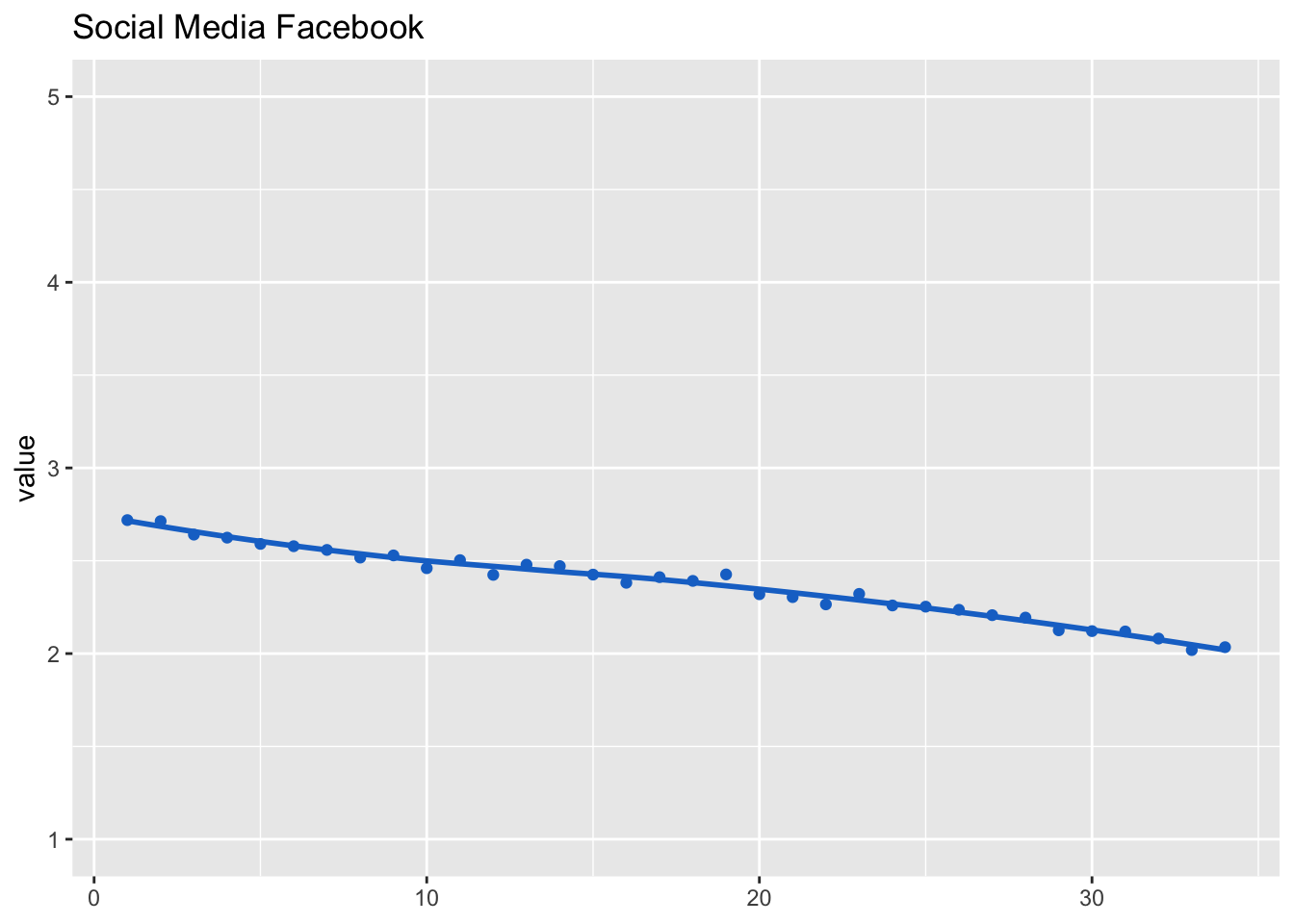

Twitter

model_soc_med_tw <- lmer(soc_med_tw ~ (1 | id) + (1 | wave), d_long_100_imp)
summary(model_soc_med_tw)

## Linear mixed model fit by REML ['lmerMod']
## Formula: soc_med_tw ~ (1 | id) + (1 | wave)
##    Data: d_long_100_imp
## 
## REML criterion at convergence: 345060
## 
## Scaled residuals: 
##    Min     1Q Median     3Q    Max 
## -2.592 -0.427 -0.257 -0.137  4.015 
## 
## Random effects:
##  Groups   Name        Variance  Std.Dev.
##  id       (Intercept) 0.0950887 0.30836 
##  wave     (Intercept) 0.0000254 0.00504 
##  Residual             0.9092064 0.95352 
## Number of obs: 123794, groups:  id, 3639; wave, 34
## 
## Fixed effects:
##             Estimate Std. Error t value
## (Intercept)  1.38753    0.00585     237

dat_fig_soc_med_tw <- data.frame(type = "Social media channel", dimension = "Twitter", 
                                 get_dat(model_soc_med_tw))
make_graph(dat_fig_soc_med_tw, "Social Media Twitter", 1, 5)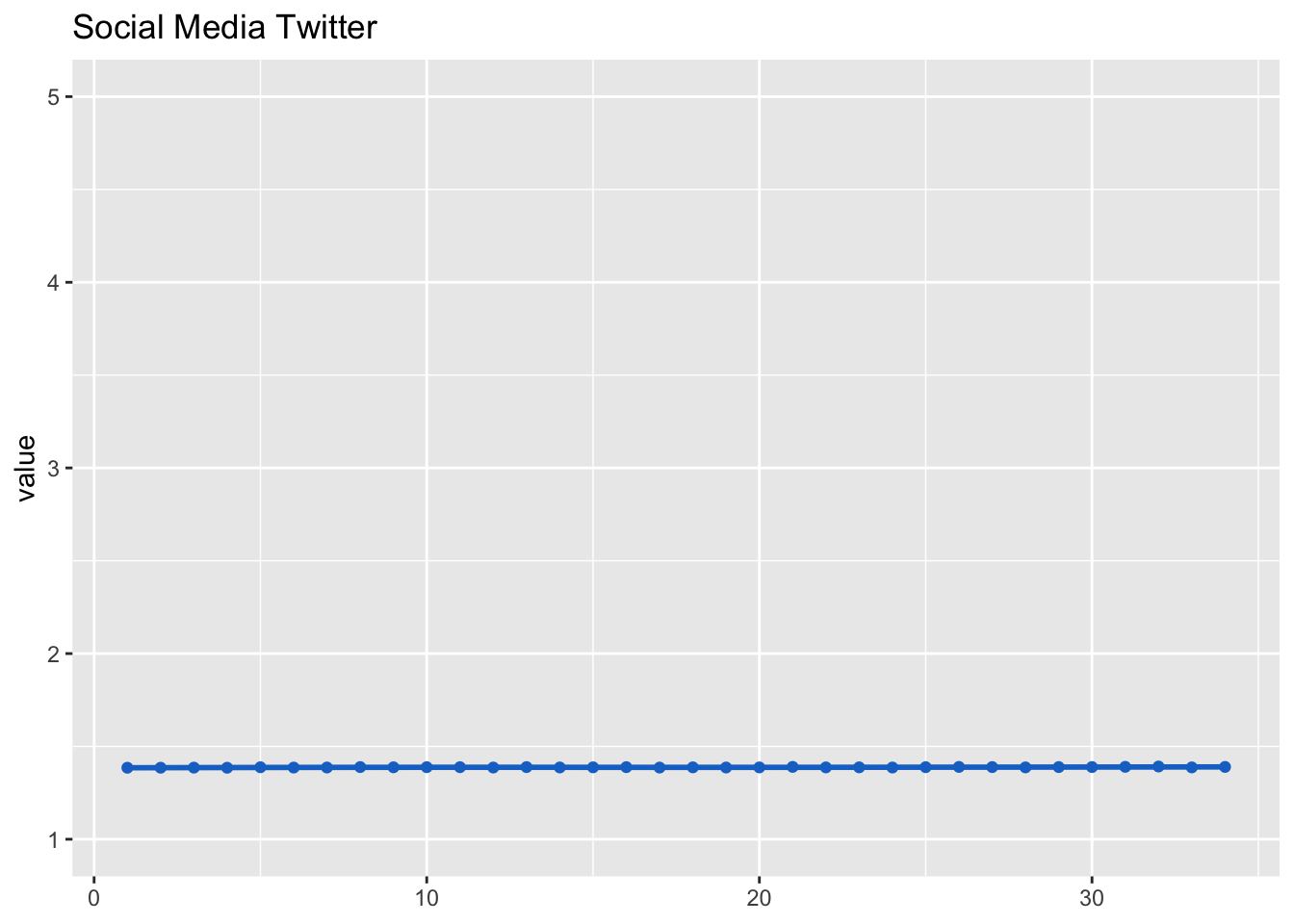

Interestingly, lme4 throws a warning, likely because there is too little variance across waves, while little variation measure itself. Let’s inspect the raw means.

soc_med_tw_m <- 
  d_long_100_imp %>% 
  group_by(wave) %>% 
  summarise(value = mean(soc_med_tw, na.rm = T))
soc_med_tw_m

ABCDEFGHIJ0123456789

wave <dbl>	value <dbl>
1	1.4
2	1.4
3	1.4
4	1.4
5	1.4
6	1.4
7	1.4
8	1.4
9	1.4
10	1.4
11	1.4
12	1.4
13	1.4
14	1.4
15	1.4
16	1.4
17	1.4
18	1.4
19	1.4
20	1.4

Inspecting the means shows that the data are intact, only that the estimation didn’t fully work.

Instagram

model_soc_med_ig <- lmer(soc_med_ig ~ (1 | id) + (1 | wave), d_long_100_imp)
summary(model_soc_med_ig)

## Linear mixed model fit by REML ['lmerMod']
## Formula: soc_med_ig ~ (1 | id) + (1 | wave)
##    Data: d_long_100_imp
## 
## REML criterion at convergence: 432311
## 
## Scaled residuals: 
##    Min     1Q Median     3Q    Max 
## -2.427 -0.568 -0.254  0.557  2.882 
## 
## Random effects:
##  Groups   Name        Variance Std.Dev.
##  id       (Intercept) 0.613791 0.7834  
##  wave     (Intercept) 0.000751 0.0274  
##  Residual             1.784792 1.3360  
## Number of obs: 123794, groups:  id, 3639; wave, 34
## 
## Fixed effects:
##             Estimate Std. Error t value
## (Intercept)   2.0463     0.0143     143

dat_fig_soc_med_ig <- data.frame(type = "Social media channel", dimension = "Instagram", 
                                 get_dat(model_soc_med_ig))
make_graph(dat_fig_soc_med_ig, "Social Media Instagram", 1, 5)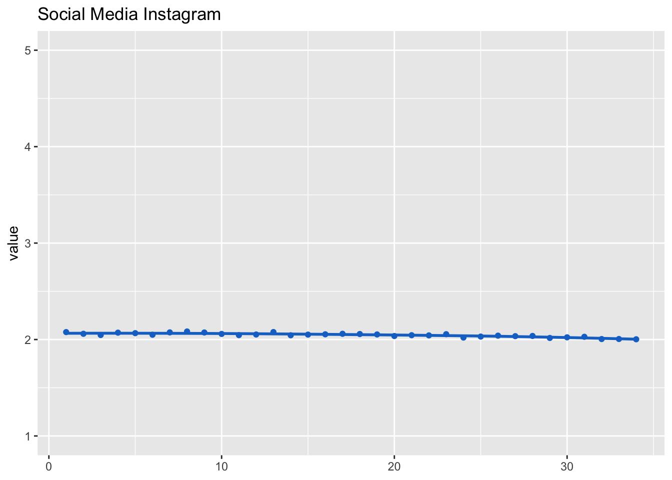

model_soc_med_wa <- lmer(soc_med_wa ~ (1 | id) + (1 | wave), d_long_100_imp)
summary(model_soc_med_wa)

## Linear mixed model fit by REML ['lmerMod']
## Formula: soc_med_wa ~ (1 | id) + (1 | wave)
##    Data: d_long_100_imp
## 
## REML criterion at convergence: 480508
## 
## Scaled residuals: 
##    Min     1Q Median     3Q    Max 
## -1.631 -0.829 -0.574  1.073  2.023 
## 
## Random effects:
##  Groups   Name        Variance Std.Dev.
##  id       (Intercept) 0.13441  0.3666  
##  wave     (Intercept) 0.00781  0.0884  
##  Residual             2.75714  1.6605  
## Number of obs: 123794, groups:  id, 3639; wave, 34
## 
## Fixed effects:
##             Estimate Std. Error t value
## (Intercept)    2.455      0.017     144

dat_fig_soc_med_wa <- data.frame(type = "Social media channel", dimension = "WhatsApp", 
                                 get_dat(model_soc_med_wa))
make_graph(dat_fig_soc_med_wa, "Social Media WhatsApp", 1, 5)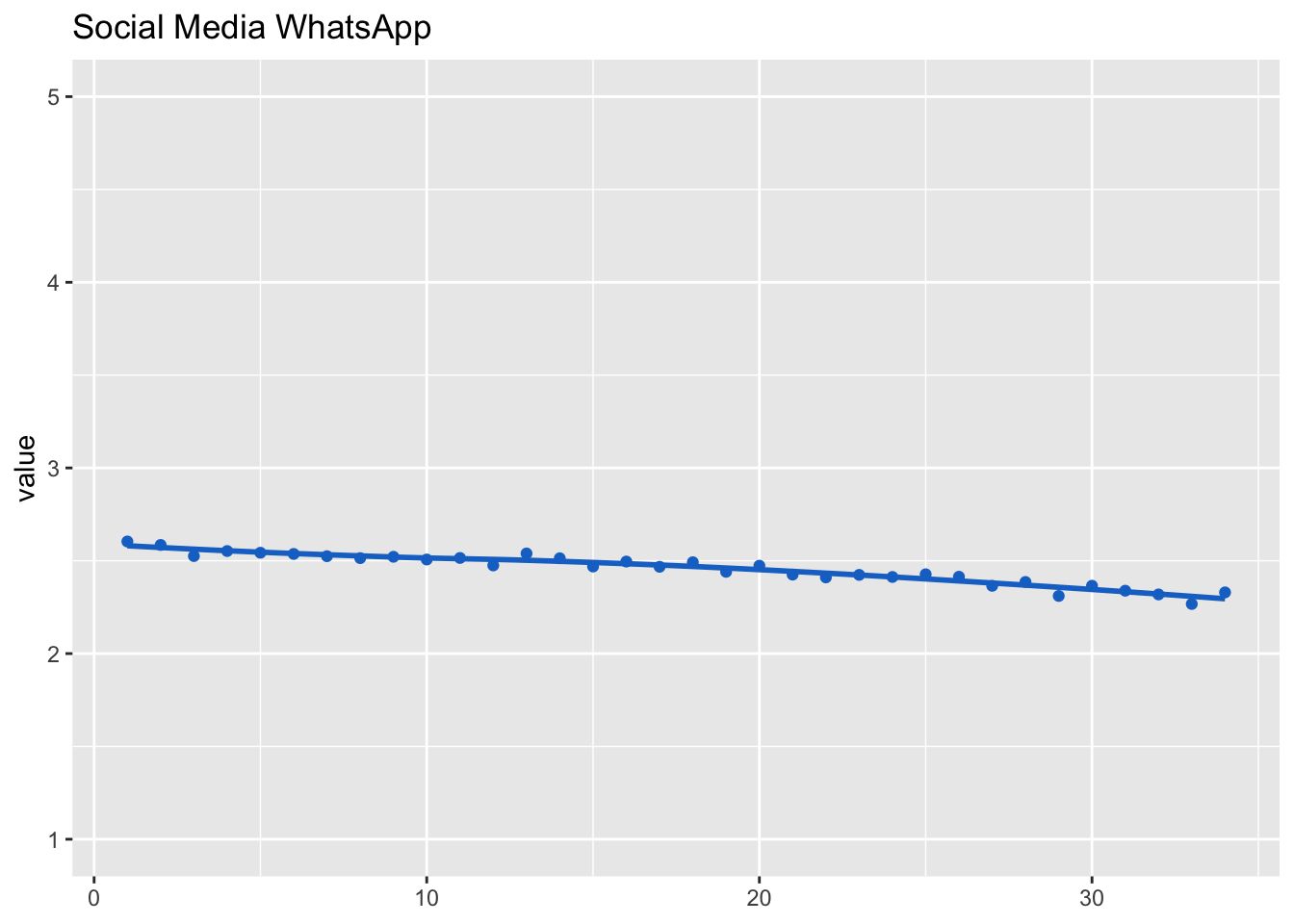

YouTube

model_soc_med_yt <- lmer(soc_med_yt ~ (1 | id) + (1 | wave), d_long_100_imp)
summary(model_soc_med_yt)

## Linear mixed model fit by REML ['lmerMod']
## Formula: soc_med_yt ~ (1 | id) + (1 | wave)
##    Data: d_long_100_imp
## 
## REML criterion at convergence: 418550
## 
## Scaled residuals: 
##    Min     1Q Median     3Q    Max 
## -2.328 -0.630 -0.370  0.542  2.955 
## 
## Random effects:
##  Groups   Name        Variance Std.Dev.
##  id       (Intercept) 0.277709 0.5270  
##  wave     (Intercept) 0.000384 0.0196  
##  Residual             1.626678 1.2754  
## Number of obs: 123794, groups:  id, 3639; wave, 34
## 
## Fixed effects:
##             Estimate Std. Error t value
## (Intercept)     1.95       0.01     194

dat_fig_soc_med_yt <- data.frame(type = "Social media channel", dimension = "YouTube", 
                                 get_dat(model_soc_med_yt))
make_graph(dat_fig_soc_med_yt, "Social Media YouTube", 1, 5)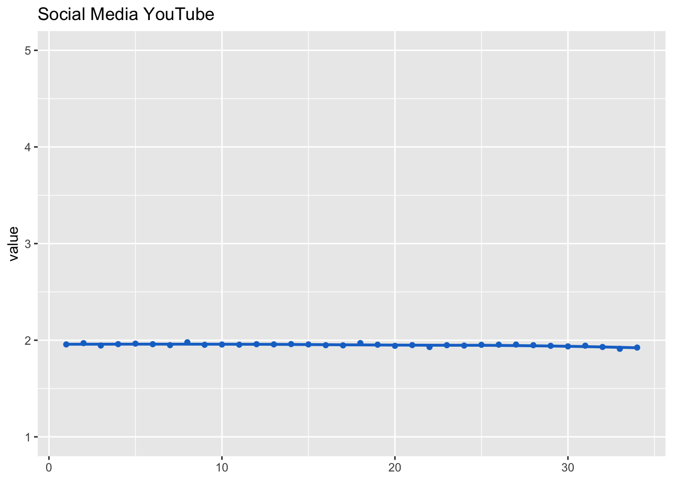

Locus of control

The only other variable that was measured as a scale was Locus of Control. Below I hence report the scale’s factorial validity. Waves for which not a sufficient number of respondents took part were excluded.

model <- "
loc_cntrl_int =~ a1*loc_cntrl_int_1 + a2*loc_cntrl_int_2 + a3*loc_cntrl_int_3 + a4*loc_cntrl_int_4
# loc_cntrl_int_1 ~~ loc_cntrl_int_2
loc_cntrl_int_3 ~~ loc_cntrl_int_4
"
cfa_loc_cntrl_int <- cfa(model, 
                         filter(d_long_100_imp, wave != 11, wave != 20,  wave != 26, wave != 27, wave != 29, wave != 31, wave != 32),
                         # d_long_100_imp,
                         group = "wave")
summary(cfa_loc_cntrl_int, standardized = TRUE, fit = TRUE, estimates = FALSE)

## lavaan 0.6.15 ended normally after 98 iterations
## 
##   Estimator                                         ML
##   Optimization method                           NLMINB
##   Number of model parameters                       351
##   Number of equality constraints                    78
## 
##   Number of observations per group:                   
##     1                                             3641
##     2                                             3641
##     3                                             3641
##     4                                             3641
##     5                                             3641
##     6                                             3641
##     7                                             3641
##     8                                             3641
##     9                                             3641
##     10                                            3641
##     12                                            3641
##     13                                            3641
##     14                                            3641
##     15                                            3641
##     16                                            3641
##     17                                            3641
##     18                                            3641
##     19                                            3641
##     21                                            3641
##     22                                            3641
##     23                                            3641
##     24                                            3641
##     25                                            3641
##     28                                            3641
##     30                                            3641
##     33                                            3641
##     34                                            3641
## 
## Model Test User Model:
##                                                       
##   Test statistic                               143.086
##   Degrees of freedom                               105
##   P-value (Chi-square)                           0.008
##   Test statistic for each group:
##     1                                            8.856
##     2                                            0.930
##     3                                            3.887
##     4                                            9.484
##     5                                            1.268
##     6                                           11.364
##     7                                            5.429
##     8                                            5.817
##     9                                            1.780
##     10                                           4.561
##     12                                           9.744
##     13                                           4.537
##     14                                          11.287
##     15                                           2.771
##     16                                           3.743
##     17                                           3.948
##     18                                           1.829
##     19                                           2.513
##     21                                          11.934
##     22                                           1.407
##     23                                           3.069
##     24                                           8.035
##     25                                           3.977
##     28                                           1.738
##     30                                           9.695
##     33                                           2.673
##     34                                           6.811
## 
## Model Test Baseline Model:
## 
##   Test statistic                             61996.667
##   Degrees of freedom                               162
##   P-value                                        0.000
## 
## User Model versus Baseline Model:
## 
##   Comparative Fit Index (CFI)                    0.999
##   Tucker-Lewis Index (TLI)                       0.999
## 
## Loglikelihood and Information Criteria:
## 
##   Loglikelihood user model (H0)            -471620.199
##   Loglikelihood unrestricted model (H1)    -471548.656
##                                                       
##   Akaike (AIC)                              943786.397
##   Bayesian (BIC)                            946378.765
##   Sample-size adjusted Bayesian (SABIC)     945511.162
## 
## Root Mean Square Error of Approximation:
## 
##   RMSEA                                          0.010
##   90 Percent confidence interval - lower         0.005
##   90 Percent confidence interval - upper         0.014
##   P-value H_0: RMSEA <= 0.050                    1.000
##   P-value H_0: RMSEA >= 0.080                    0.000
## 
## Standardized Root Mean Square Residual:
## 
##   SRMR                                           0.011

The data fit the model very well, $\chi^2$ (105) = 143.09, p = .008, CFI = 1.00, RMSEA < .01, 90% CI [.01, .01], SRMR = .01.

Table

Table with descriptives of main variables.

tab_desc_dat <- rbind(
    "Life satisfaction" = get_specs(fit_life_sat),
    "Positive affect" = get_specs(model_aff_pos),
    "Negative affect" = get_specs(model_aff_neg),
    "Read" = get_specs(model_soc_med_read),
    "Like & share" = get_specs(model_soc_med_like_share),
    "Posting" = get_specs(model_soc_med_post),
    "Facebook" = get_specs(model_soc_med_fb),
    "Twitter" = c(sd = get_specs(model_soc_med_tw)$sd,
                  min = min(soc_med_tw_m$value, na.rm = TRUE),
                  max = max(soc_med_tw_m$value, na.rm = TRUE),
                  mean = mean(soc_med_tw_m$value, na.rm = TRUE)
                  ),
    "Instagram" = get_specs(model_soc_med_ig),
    "WhatsApp" = get_specs(model_soc_med_wa),
    "YouTube" = get_specs(model_soc_med_yt)
    ) %>%
  as.data.frame()
tab_desc_dat

ABCDEFGHIJ0123456789

	sd <dbl>	min <dbl>	max <dbl>	mean <dbl>
Life satisfaction	2.23	6.3	6.6	6.5
Positive affect	0.94	3.1	3.2	3.2
Negative affect	0.77	1.8	1.9	1.8
Read	1.38	1.9	2.9	2.4
Like & share	1.19	1.5	1.9	1.7
Posting	0.89	1.4	1.4	1.4
Facebook	1.58	2.0	2.7	2.4
Twitter	0.95	1.4	1.4	1.4
Instagram	1.34	2.0	2.1	2.0
WhatsApp	1.66	2.3	2.6	2.5
YouTube	1.28	1.9	2.0	2.0

Figure

Display the developments of all variables in a combined figure.

fig_desc_dat <- data.frame(
  rbind(
    dat_fig_life_sat,
    dat_fig_aff_pos,
    dat_fig_aff_neg,
    dat_fig_soc_med_read,
    dat_fig_soc_med_like_share,
    dat_fig_soc_med_post,
    dat_fig_soc_med_fb,
    dat_fig_soc_med_tw,
    dat_fig_soc_med_ig,
    dat_fig_soc_med_wa,
    dat_fig_soc_med_yt
  ) %>% 
    mutate(
      type = factor(.$type, levels = c("Life satisfaction", "Affect", "Social media use", "Social media channel")),
      dimension = factor(.$dimension, levels = c("Life satisfaction", "Positive", "Negative", "Reading", "Liking & Sharing", "Posting", "Facebook", "Twitter", "Instagram", "WhatsApp", "YouTube"))
      )
)

fig_desc_life_sat <- make_graph(
  fig_desc_dat %>% filter(type == "Life satisfaction"), 
  title = "Life satisfaction", 
  ll = 0, ul = 10, 
  lmer = FALSE, 
  line = TRUE,
  legend = FALSE,
  points = FALSE
  )

fig_desc_aff <- make_graph(
  fig_desc_dat %>% filter(type == "Affect"), 
  title = "Affect", 
  ll = 1, ul = 5, 
  lmer = FALSE, 
  line = TRUE,
  points = FALSE,
  legend = TRUE
  )

fig_desc_soc_med_use <- make_graph(
  fig_desc_dat %>% filter(type == "Social media use"), 
  title = "Social media use", 
  ll = 1, ul = 5, 
  lmer = FALSE, 
  line = TRUE,
  points = FALSE,
  legend = TRUE
  )

fig_desc_soc_med_channel <- make_graph(
  fig_desc_dat %>% filter(type == "Social media channel"), 
  title = "Social media channel", 
  ll = 1, ul = 5, 
  lmer = FALSE, 
  line = TRUE,
  points = FALSE,
  legend = TRUE
  )

fig_desc <- grid.arrange(fig_desc_life_sat, fig_desc_aff, 
                         fig_desc_soc_med_use, fig_desc_soc_med_channel,
                         nrow = 2, ncol = 2)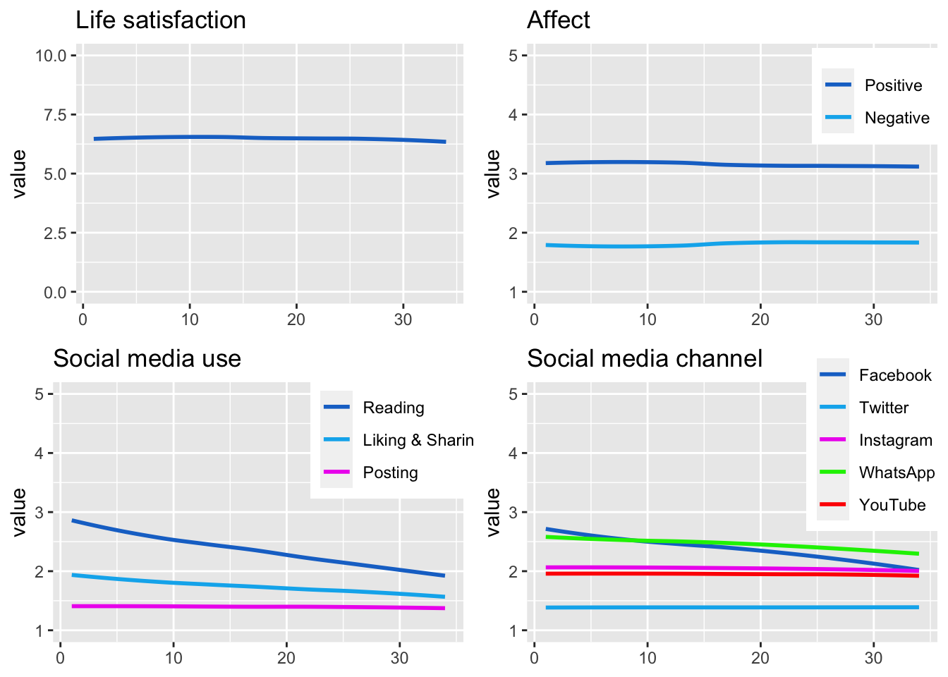

ggsave("figures/fig_descriptives.png", 
       width = 10, height = 5,
       plot = fig_desc)

Analyses

Multicollinearity

Before running the analyses, let’s briefly check zero-order correlation matrix, to get general picture and also for potential multicollinearity. We use variables from T1.

Multicollinearity will then also be checked explicitly in each analysis.

d_long_100_imp %>% 
  filter(wave == 1) %>% 
  select(life_sat, aff_neg_m, aff_pos_m,
         soc_med_read, soc_med_post, soc_med_like_share, 
         soc_med_fb, soc_med_ig, soc_med_tw, soc_med_wa, soc_med_yt,
         health, corona_pos, work_h, work_homeoff, hh_income, med_txt_kro, med_txt_sta, med_txt_pre, med_txt_oes, med_txt_kur, med_txt_slz, med_txt_son, med_vid_orf, med_vid_pri, med_txt_kro, med_txt_sta, med_txt_pre, med_txt_oes, med_txt_kur, med_txt_slz, med_txt_son, med_vid_orf, med_vid_pri, act_wrk, act_spo, act_frn, act_sho, act_pet, risk_prop, loc_cntrl_int_m, sat_dem) %>% 
  cor(use = "pairwise.complete.obs") %>% 
  as.data.frame()

ABCDEFGHIJ0123456789

	life_sat <dbl>	aff_neg_m <dbl>	aff_pos_m <dbl>	soc_med_read <dbl>	soc_med_post <dbl>	soc_med_like_share <dbl>	soc_med_fb <dbl>	soc_med_ig <dbl>
life_sat	1.00000	-0.396	0.3708	-0.0023	-0.085	-0.0696	0.0079	-0.0097
aff_neg_m	-0.39616	1.000	-0.4220	0.1394	0.269	0.2142	0.1067	0.2118
aff_pos_m	0.37081	-0.422	1.0000	-0.0640	-0.056	-0.0664	-0.0194	-0.0387
soc_med_read	-0.00231	0.139	-0.0640	1.0000	0.320	0.5343	0.5162	0.3351
soc_med_post	-0.08540	0.269	-0.0557	0.3204	1.000	0.5310	0.2323	0.2376
soc_med_like_share	-0.06958	0.214	-0.0664	0.5343	0.531	1.0000	0.3781	0.3263
soc_med_fb	0.00793	0.107	-0.0194	0.5162	0.232	0.3781	1.0000	0.3554
soc_med_ig	-0.00971	0.212	-0.0387	0.3351	0.238	0.3263	0.3554	1.0000
soc_med_tw	-0.07728	0.222	-0.0402	0.2464	0.372	0.3122	0.1534	0.3304
soc_med_wa	-0.01419	0.133	0.0166	0.3221	0.226	0.2768	0.4460	0.4150
soc_med_yt	-0.06835	0.225	-0.0356	0.2532	0.296	0.2881	0.2796	0.4605
health	0.32979	-0.329	0.3375	-0.0060	-0.082	-0.0806	0.0235	0.0367
corona_pos	0.01160	-0.070	0.0090	0.0147	-0.032	0.0148	-0.0071	-0.0176
work_h	0.07082	-0.085	0.0835	-0.0670	-0.052	-0.0657	-0.0459	-0.0015
work_homeoff	0.04593	-0.037	0.0120	0.0183	-0.026	0.0046	-0.0216	0.0941
hh_income	0.19845	-0.166	0.1156	0.0046	-0.082	-0.0595	-0.0450	-0.0149
med_txt_kro	-0.00890	0.071	-0.0116	0.0927	0.095	0.0939	0.1304	0.0169
med_txt_sta	0.00049	0.122	-0.0422	0.1947	0.164	0.1912	0.0866	0.2427
med_txt_pre	-0.02660	0.161	-0.0188	0.1947	0.225	0.2218	0.0891	0.2259
med_txt_oes	-0.08080	0.163	-0.0387	0.1301	0.169	0.1600	0.1364	0.0738

Correlations

Let’s also briefly look at bivariate relations between the types and channels of social media use and the well-being facets.

Table

dat_cor <- 
  d_long_100_mim %>% 
  filter(wave == 1) %>%  # we can use wave 1 only, because mean values are the same across waves
  select(`Life satis-\nfaction` = life_sat_b, 
         `Affect\npositive` = aff_pos_m_b, 
         `Affect\nnegative` = aff_neg_m_b,
         `Reading` = soc_med_read_b, 
         `Posting` = soc_med_post_b, 
         `Like &\nshare` = soc_med_like_share_b, 
         `Facebook` = soc_med_fb_b, 
         `Instagram` = soc_med_ig_b, 
         `Twitter` = soc_med_tw_b, 
         `WhatsApp` = soc_med_wa_b, 
         `YouTube` = soc_med_yt_b)
  # cor() %>% 
  # as.data.frame()
  # correlate() %>% 
  # fashion()

tab_cor <- 
  dat_cor %>% 
  correlate() %>% 
  fashion() %T>%
  print()

##                    term Life.satis..faction Affect.positive Affect.negative Reading Posting Like...share Facebook Instagram Twitter WhatsApp YouTube
## 1  Life satis-\nfaction                                 .61            -.55    -.10    -.25         -.21     -.11      -.01    -.14     -.03    -.13
## 2      Affect\npositive                 .61                            -.48    -.15    -.03         -.13     -.07      -.01     .02      .01     .00
## 3      Affect\nnegative                -.55            -.48                     .52     .61          .61      .32       .49     .52      .43     .55
## 4               Reading                -.10            -.15             .52             .50          .79      .45       .79     .50      .47     .58
## 5               Posting                -.25            -.03             .61     .50                  .78      .35       .53     .77      .62     .77
## 6         Like &\nshare                -.21            -.13             .61     .79     .78                   .34       .72     .66      .63     .73
## 7              Facebook                -.11            -.07             .32     .45     .35          .34                .25     .19      .44     .30
## 8             Instagram                -.01            -.01             .49     .79     .53          .72      .25               .64      .57     .79
## 9               Twitter                -.14             .02             .52     .50     .77          .66      .19       .64              .51     .78
## 10             WhatsApp                -.03             .01             .43     .47     .62          .63      .44       .57     .51              .69
## 11              YouTube                -.13             .00             .55     .58     .77          .73      .30       .79     .78      .69

Figure

int_breaks <- function(x, n = 4) {
  l <- pretty(x, n)
  l[abs(l %% 1) < .Machine$double.eps ^ 0.5] 
}

fig_cor <- 
  dat_cor %>% 
  ggpairs(
    upper = list(continuous = cor_plot),
    lower = list(continuous = wrap("points", alpha = 0.3, size=0.1), 
              combo = wrap("dot", alpha = 0.3, size=0.1)),
    progress = FALSE
    ) + 
  scale_x_continuous(breaks = int_breaks) +
  theme_bw()

fig_cor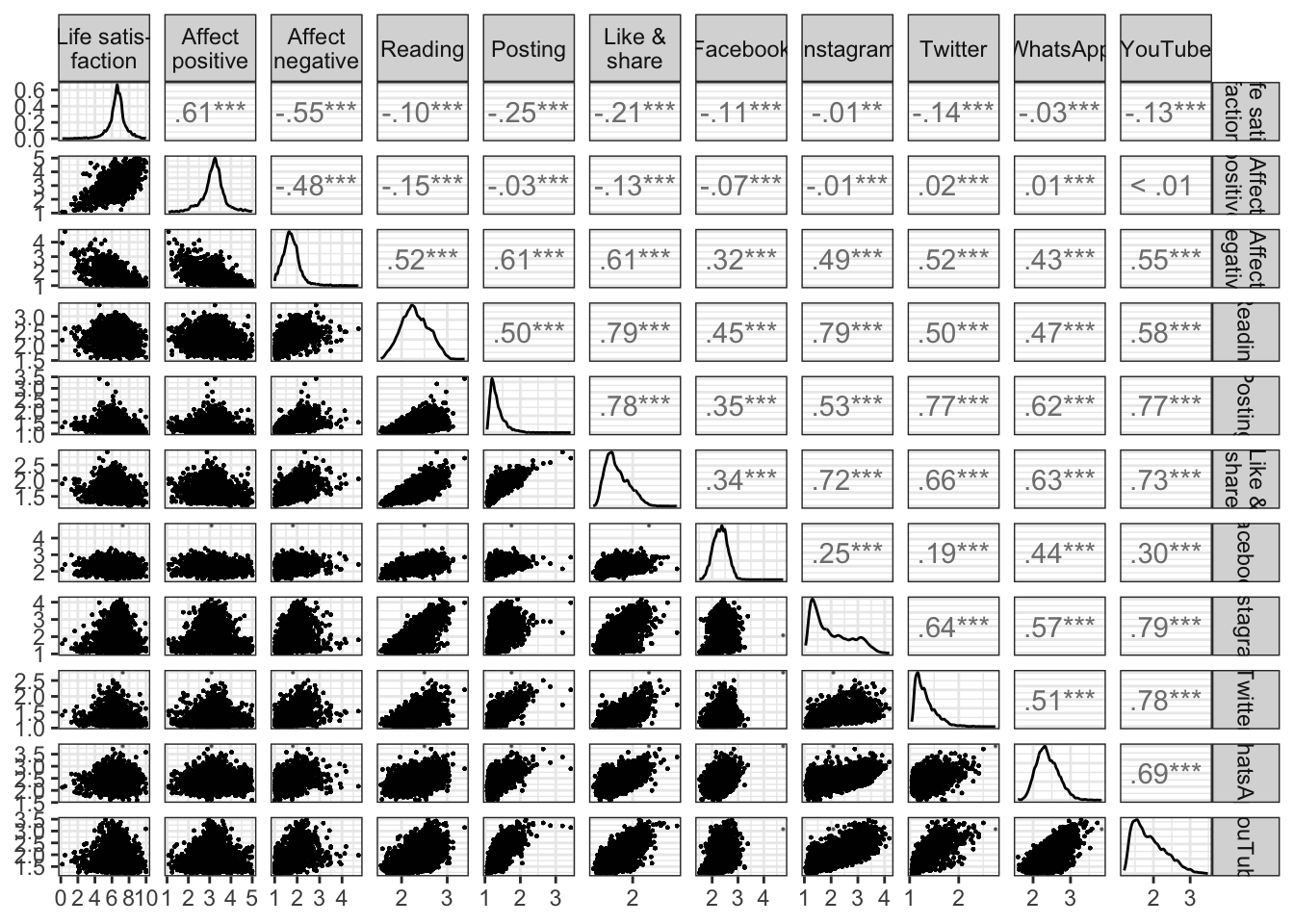

ggsave("figures/fig_cor.png", width = 8, height = 8)

Publication

Life satisfaction

model_life_sat_lmer_pub <- "
  life_sat ~ 
    (1 | id) + (1 | wave) + 
    soc_med_read_w + soc_med_like_share_w + soc_med_post_w  + 
    soc_med_fb_w + soc_med_ig_w + soc_med_wa_w + soc_med_yt_w + soc_med_tw_w +
    soc_med_read_b + soc_med_like_share_b + soc_med_post_b + 
    soc_med_fb_b + soc_med_ig_b + soc_med_wa_b + soc_med_yt_b + soc_med_tw_b +  
    age + male + born_aus + born_aus_prnts + edu_fac + employment_fac +
    res_vienna + acc_bal + acc_gar + home_sqm + 
    corona_pos_b + corona_pos_w +
    work_h_b + work_h_w +
    work_homeoff_b +  work_homeoff_w +
    hh_income_b + hh_income_w +
    hh_adults + hh_child18 + hh_child17 + hh_child14 + hh_child5 + hh_child2 + 
    hh_oldfam + hh_outfam + hh_partner +
    home_owner +
    risk_prop_b + risk_prop_w + 
    act_wrk_w + act_spo_w + act_frn_w + act_sho_w + act_pet_w + 
    act_wrk_b + act_spo_b + act_frn_b + act_sho_b + act_pet_b +
    health_w + health_b +
    loc_cntrl_int_m_w + loc_cntrl_int_m_b
"

Let’s first inspect multicollinearity.

check_collinearity(lmerTest::lmer(model_life_sat_lmer_pub, d_long_100_imp))

ABCDEFGHIJ0123456789

Term <chr>	VIF <dbl>	VIF_CI_low <dbl>	VIF_CI_high <dbl>	SE_factor <dbl>	Tolerance <dbl>	Tolerance_CI_low <dbl>	Tolerance_CI_high <dbl>
soc_med_read_w	1.7	1.7	1.8	1.3	0.572	0.567	0.576
soc_med_like_share_w	1.9	1.9	1.9	1.4	0.518	0.513	0.522
soc_med_post_w	1.6	1.6	1.6	1.3	0.614	0.609	0.619
soc_med_fb_w	1.6	1.6	1.6	1.3	0.619	0.614	0.624
soc_med_ig_w	1.4	1.4	1.5	1.2	0.691	0.686	0.696
soc_med_wa_w	1.7	1.7	1.7	1.3	0.591	0.586	0.595
soc_med_yt_w	1.6	1.6	1.6	1.3	0.617	0.612	0.622
soc_med_tw_w	1.3	1.3	1.3	1.2	0.753	0.748	0.758
soc_med_read_b	5.1	5.1	5.2	2.3	0.195	0.193	0.197
soc_med_like_share_b	7.0	6.9	7.1	2.6	0.143	0.141	0.144
soc_med_post_b	6.4	6.3	6.4	2.5	0.157	0.156	0.159
soc_med_fb_b	3.1	3.1	3.1	1.8	0.322	0.319	0.325
soc_med_ig_b	11.4	11.3	11.6	3.4	0.087	0.086	0.088
soc_med_wa_b	3.6	3.6	3.6	1.9	0.277	0.275	0.280
soc_med_yt_b	9.0	8.9	9.1	3.0	0.111	0.109	0.112
soc_med_tw_b	4.3	4.3	4.3	2.1	0.233	0.231	0.235
age	9.4	9.3	9.5	3.1	0.107	0.105	0.108
male	3.3	3.3	3.4	1.8	0.301	0.298	0.304
born_aus	1.2	1.2	1.2	1.1	0.806	0.801	0.811
born_aus_prnts	1.6	1.6	1.6	1.3	0.624	0.619	0.629

No within-person predictor shows increased values for multicollinearity. Hence results straightforward.

Let’s next inspect results of within-person predictors. Only parts of model shown to save space.

fit_life_sat_lmer_pub <- with(d_long_100_mim_mice, exp = lmerTest::lmer(model_life_sat_lmer_pub))
fit_life_sat_lmer_pub <- summary(pool(fit_life_sat_lmer_pub), conf.int = TRUE)
print_res(fit_life_sat_lmer_pub)

ABCDEFGHIJ0123456789

term <fct>	estimate <dbl>	2.5 % <dbl>	97.5 % <dbl>	p.value <chr>
(Intercept)	-4.62691	-5.53347	-3.7204	< .001
soc_med_read_w	0.01002	-0.03369	0.0537	.639
soc_med_like_share_w	-0.02248	-0.05982	0.0149	.227
soc_med_post_w	-0.04471	-0.08342	-0.0060	.025
soc_med_fb_w	-0.00969	-0.04085	0.0215	.527
soc_med_ig_w	0.02896	-0.01116	0.0691	.149
soc_med_wa_w	-0.00189	-0.03894	0.0352	.917
soc_med_yt_w	0.00617	-0.02798	0.0403	.713
soc_med_tw_w	-0.01345	-0.05418	0.0273	.503
soc_med_read_b	0.03973	-0.21241	0.2919	.757
soc_med_like_share_b	-0.04810	-0.37528	0.2791	.773
soc_med_post_b	0.02462	-0.32552	0.3747	.890
soc_med_fb_b	-0.25290	-0.40919	-0.0966	.002
soc_med_ig_b	-0.10348	-0.26919	0.0622	.220
soc_med_wa_b	0.37884	0.19150	0.5662	< .001
soc_med_yt_b	0.08911	-0.11917	0.2974	.401
soc_med_tw_b	0.38143	0.12239	0.6405	.004
age	-0.00092	-0.00734	0.0055	.776
male	-0.09945	-0.20178	0.0029	.057
born_aus	-0.09839	-0.20511	0.0083	.070

Positive Affect

model_aff_pos_lmer_pub <- "
  aff_pos_m ~ 
    (1 | id) + (1 | wave) + 
    soc_med_read_w + soc_med_like_share_w + soc_med_post_w  + 
    soc_med_fb_w + soc_med_ig_w + soc_med_wa_w + soc_med_yt_w + soc_med_tw_w +
    soc_med_read_b + soc_med_like_share_b + soc_med_post_b + 
    soc_med_fb_b + soc_med_ig_b + soc_med_wa_b + soc_med_yt_b + soc_med_tw_b +  
    age + male + born_aus + born_aus_prnts + edu_fac + employment_fac +
    res_vienna + acc_bal + acc_gar + home_sqm + 
    corona_pos_b + corona_pos_w +
    work_h_b + work_h_w +
    work_homeoff_b +  work_homeoff_w +
    hh_income_b + hh_income_w +
    hh_adults + hh_child18 + hh_child17 + hh_child14 + hh_child5 + hh_child2 + 
    hh_oldfam + hh_outfam + hh_partner +
    home_owner +
    risk_prop_b + risk_prop_w + 
    act_wrk_w + act_spo_w + act_frn_w + act_sho_w + act_pet_w + 
    act_wrk_b + act_spo_b + act_frn_b + act_sho_b + act_pet_b +
    health_w + health_b +
    loc_cntrl_int_m_w + loc_cntrl_int_m_b
"

Let’s first inspect multicollinearity.

check_collinearity(lmerTest::lmer(model_aff_pos_lmer_pub, d_long_100_imp))

ABCDEFGHIJ0123456789

Term <chr>	VIF <dbl>	VIF_CI_low <dbl>	VIF_CI_high <dbl>	SE_factor <dbl>	Tolerance <dbl>	Tolerance_CI_low <dbl>	Tolerance_CI_high <dbl>
soc_med_read_w	1.7	1.7	1.8	1.3	0.575	0.570	0.580
soc_med_like_share_w	1.9	1.9	1.9	1.4	0.519	0.515	0.524
soc_med_post_w	1.6	1.6	1.6	1.3	0.614	0.609	0.619
soc_med_fb_w	1.6	1.6	1.6	1.3	0.622	0.617	0.627
soc_med_ig_w	1.4	1.4	1.5	1.2	0.691	0.686	0.696
soc_med_wa_w	1.7	1.7	1.7	1.3	0.591	0.586	0.596
soc_med_yt_w	1.6	1.6	1.6	1.3	0.617	0.612	0.622
soc_med_tw_w	1.3	1.3	1.3	1.2	0.753	0.747	0.758
soc_med_read_b	5.1	5.0	5.1	2.3	0.196	0.194	0.198
soc_med_like_share_b	6.9	6.9	7.0	2.6	0.144	0.142	0.145
soc_med_post_b	6.3	6.2	6.3	2.5	0.160	0.158	0.161
soc_med_fb_b	3.0	3.0	3.0	1.7	0.332	0.329	0.335
soc_med_ig_b	10.9	10.8	11.0	3.3	0.092	0.091	0.093
soc_med_wa_b	3.5	3.5	3.6	1.9	0.282	0.280	0.285
soc_med_yt_b	8.9	8.8	9.0	3.0	0.112	0.111	0.113
soc_med_tw_b	4.2	4.2	4.2	2.0	0.238	0.236	0.240
age	9.1	9.0	9.2	3.0	0.110	0.109	0.111
male	3.3	3.2	3.3	1.8	0.305	0.302	0.308
born_aus	1.2	1.2	1.2	1.1	0.810	0.805	0.816
born_aus_prnts	1.6	1.6	1.6	1.3	0.635	0.630	0.640

No within-person predictors show multicollinear relations.

In what follows, the results of within-person predictors.

fit_aff_pos_lmer_pub <- with(d_long_100_mim_mice, exp = lmerTest::lmer(model_aff_pos_lmer_pub))
fit_aff_pos_lmer_pub <- summary(pool(fit_aff_pos_lmer_pub), conf.int = TRUE)
print_res(fit_aff_pos_lmer_pub)

ABCDEFGHIJ0123456789

term <fct>	estimate <dbl>	2.5 % <dbl>	97.5 % <dbl>	p.value <chr>
(Intercept)	-3.40553	-3.8123	-2.998778	< .001
soc_med_read_w	-0.03189	-0.0474	-0.016363	< .001
soc_med_like_share_w	0.00555	-0.0115	0.022549	.508
soc_med_post_w	0.02411	0.0090	0.039224	.003
soc_med_fb_w	-0.00259	-0.0150	0.009848	.671
soc_med_ig_w	-0.00616	-0.0207	0.008372	.390
soc_med_wa_w	0.00601	-0.0077	0.019749	.374
soc_med_yt_w	0.00297	-0.0120	0.017939	.686
soc_med_tw_w	0.01315	-0.0041	0.030437	.130
soc_med_read_b	-0.51606	-0.6275	-0.404644	< .001
soc_med_like_share_b	0.28864	0.1396	0.437679	< .001
soc_med_post_b	0.73540	0.5770	0.893827	< .001
soc_med_fb_b	-0.15521	-0.2279	-0.082564	< .001
soc_med_ig_b	-0.09117	-0.1635	-0.018862	.014
soc_med_wa_b	0.10960	0.0226	0.196565	.014
soc_med_yt_b	0.04950	-0.0562	0.155193	.358
soc_med_tw_b	-0.03258	-0.1531	0.087931	.595
age	-0.00774	-0.0105	-0.004955	< .001
male	0.07562	0.0223	0.128919	.006
born_aus	0.06660	0.0121	0.121107	.017

Negative Affect

model_aff_neg_lmer_pub <- "
  aff_neg_m ~ 
    (1 | id) + (1 | wave) + 
    soc_med_read_w + soc_med_like_share_w + soc_med_post_w  + 
    soc_med_fb_w + soc_med_ig_w + soc_med_wa_w + soc_med_yt_w + soc_med_tw_w +
    soc_med_read_b + soc_med_like_share_b + soc_med_post_b + 
    soc_med_fb_b + soc_med_ig_b + soc_med_wa_b + soc_med_yt_b + soc_med_tw_b +  
    age + male + born_aus + born_aus_prnts + edu_fac + employment_fac +
    res_vienna + acc_bal + acc_gar + home_sqm + 
    corona_pos_b + corona_pos_w +
    work_h_b + work_h_w +
    work_homeoff_b +  work_homeoff_w +
    hh_income_b + hh_income_w +
    hh_adults + hh_child18 + hh_child17 + hh_child14 + hh_child5 + hh_child2 + 
    hh_oldfam + hh_outfam + hh_partner +
    home_owner +
    risk_prop_b + risk_prop_w + 
    act_wrk_w + act_spo_w + act_frn_w + act_sho_w + act_pet_w + 
    act_wrk_b + act_spo_b + act_frn_b + act_sho_b + act_pet_b +
    health_w + health_b +
    loc_cntrl_int_m_w + loc_cntrl_int_m_b
"

Let’s inspect multicollinearity.

check_collinearity(lmerTest::lmer(model_aff_neg_lmer_pub, d_long_100_imp))

ABCDEFGHIJ0123456789

Term <chr>	VIF <dbl>	VIF_CI_low <dbl>	VIF_CI_high <dbl>	SE_factor <dbl>	Tolerance <dbl>	Tolerance_CI_low <dbl>	Tolerance_CI_high <dbl>
soc_med_read_w	1.7	1.7	1.8	1.3	0.574	0.570	0.579
soc_med_like_share_w	1.9	1.9	1.9	1.4	0.519	0.514	0.523
soc_med_post_w	1.6	1.6	1.6	1.3	0.614	0.609	0.619
soc_med_fb_w	1.6	1.6	1.6	1.3	0.621	0.616	0.626
soc_med_ig_w	1.4	1.4	1.5	1.2	0.691	0.686	0.696
soc_med_wa_w	1.7	1.7	1.7	1.3	0.591	0.586	0.596
soc_med_yt_w	1.6	1.6	1.6	1.3	0.617	0.612	0.622
soc_med_tw_w	1.3	1.3	1.3	1.2	0.753	0.747	0.758
soc_med_read_b	5.1	5.1	5.2	2.3	0.195	0.193	0.197
soc_med_like_share_b	7.0	6.9	7.1	2.6	0.143	0.141	0.144
soc_med_post_b	6.3	6.3	6.4	2.5	0.158	0.156	0.159
soc_med_fb_b	3.1	3.1	3.1	1.8	0.323	0.320	0.326
soc_med_ig_b	11.4	11.3	11.5	3.4	0.088	0.087	0.089
soc_med_wa_b	3.6	3.6	3.6	1.9	0.278	0.275	0.281
soc_med_yt_b	9.0	8.9	9.1	3.0	0.111	0.110	0.112
soc_med_tw_b	4.3	4.2	4.3	2.1	0.233	0.231	0.236
age	9.4	9.3	9.5	3.1	0.107	0.106	0.108
male	3.3	3.3	3.4	1.8	0.301	0.298	0.304
born_aus	1.2	1.2	1.2	1.1	0.807	0.801	0.812
born_aus_prnts	1.6	1.6	1.6	1.3	0.625	0.620	0.630

No within-person predictors show multicollinear relations.

Here are the results for the within-person predictors.

fit_aff_neg_lmer_pub <- with(d_long_100_mim_mice, exp = lmerTest::lmer(model_aff_neg_lmer_pub))
fit_aff_neg_lmer_pub <- summary(pool(fit_aff_neg_lmer_pub), conf.int = TRUE)
print_res(fit_aff_neg_lmer_pub)

ABCDEFGHIJ0123456789

term <fct>	estimate <dbl>	2.5 % <dbl>	97.5 % <dbl>	p.value <chr>
(Intercept)	4.08332	3.82017	4.346477	< .001
soc_med_read_w	0.00217	-0.01164	0.015990	.747
soc_med_like_share_w	0.02014	0.00324	0.037040	.022
soc_med_post_w	0.05295	0.03562	0.070287	< .001
soc_med_fb_w	-0.00228	-0.01482	0.010266	.710
soc_med_ig_w	-0.00274	-0.01523	0.009752	.654
soc_med_wa_w	0.00377	-0.00567	0.013219	.417
soc_med_yt_w	0.01400	0.00354	0.024457	.011
soc_med_tw_w	0.02497	0.00723	0.042708	.008
soc_med_read_b	0.12637	0.04843	0.204314	.002
soc_med_like_share_b	0.19499	0.09976	0.290227	< .001
soc_med_post_b	0.30372	0.19594	0.411495	< .001
soc_med_fb_b	0.04154	-0.01141	0.094490	.124
soc_med_ig_b	0.03601	-0.01527	0.087282	.168
soc_med_wa_b	0.02792	-0.02899	0.084824	.335
soc_med_yt_b	0.04052	-0.03129	0.112329	.268
soc_med_tw_b	-0.02315	-0.10227	0.055978	.565
age	-0.00182	-0.00377	0.000126	.067
male	-0.04704	-0.08011	-0.013968	.005
born_aus	-0.01691	-0.05105	0.017237	.328

Standardized results

Then let’s report also the standardized results. Helps compare effect sizes across differently scaled predictors.

Life satisfaction

fit_life_sat_lmer_std <- with(d_long_100_mim_mice_std, exp = lmerTest::lmer(model_life_sat_lmer_pub))
fit_life_sat_lmer_std <- summary(pool(fit_life_sat_lmer_std), conf.int = TRUE)
print_res(fit_life_sat_lmer_std)

ABCDEFGHIJ0123456789

term <fct>	estimate <dbl>	2.5 % <dbl>	97.5 % <dbl>	p.value <chr>
(Intercept)	0.6741	0.55633	0.7919	< .001
soc_med_read_w	0.0054	-0.02060	0.0314	.671
soc_med_like_share_w	-0.0110	-0.02962	0.0076	.234
soc_med_post_w	-0.0155	-0.02953	-0.0016	.030
soc_med_fb_w	-0.0063	-0.02721	0.0146	.538
soc_med_ig_w	0.0175	-0.00781	0.0428	.166
soc_med_wa_w	-0.0010	-0.02717	0.0251	.935
soc_med_yt_w	0.0032	-0.01597	0.0224	.733
soc_med_tw_w	-0.0045	-0.01987	0.0108	.547
soc_med_read_b	0.0182	-0.13110	0.1676	.810
soc_med_like_share_b	-0.0238	-0.18568	0.1380	.772
soc_med_post_b	0.0185	-0.10615	0.1432	.770
soc_med_fb_b	-0.1655	-0.27087	-0.0602	.002
soc_med_ig_b	-0.0637	-0.16786	0.0404	.229
soc_med_wa_b	0.2627	0.13209	0.3933	< .001
soc_med_yt_b	0.0517	-0.06386	0.1673	.380
soc_med_tw_b	0.1477	0.05139	0.2441	.003
age	-0.0074	-0.05424	0.0394	.754
male	-0.0375	-0.08020	0.0051	.084
born_aus	-0.0432	-0.08787	0.0015	.058

Positive Affect

fit_aff_pos_lmer_std <- with(d_long_100_mim_mice_std, exp = lmerTest::lmer(model_aff_pos_lmer_pub))
fit_aff_pos_lmer_std <- summary(pool(fit_aff_pos_lmer_std), conf.int = TRUE)
print_res(fit_aff_pos_lmer_std)

ABCDEFGHIJ0123456789

term <fct>	estimate <dbl>	2.5 % <dbl>	97.5 % <dbl>	p.value <chr>
(Intercept)	0.4694	0.3514	0.58747	< .001
soc_med_read_w	-0.0381	-0.0562	-0.01997	< .001
soc_med_like_share_w	0.0056	-0.0110	0.02229	.492
soc_med_post_w	0.0175	0.0067	0.02834	.002
soc_med_fb_w	-0.0034	-0.0198	0.01302	.674
soc_med_ig_w	-0.0080	-0.0259	0.01001	.369
soc_med_wa_w	0.0084	-0.0106	0.02742	.369
soc_med_yt_w	0.0032	-0.0132	0.01964	.691
soc_med_tw_w	0.0104	-0.0027	0.02345	.115
soc_med_read_b	-0.6069	-0.7371	-0.47658	< .001
soc_med_like_share_b	0.2853	0.1397	0.43093	< .001
soc_med_post_b	0.5328	0.4205	0.64507	< .001
soc_med_fb_b	-0.2050	-0.3012	-0.10866	< .001
soc_med_ig_b	-0.1175	-0.2077	-0.02723	.011
soc_med_wa_b	0.1578	0.0378	0.27785	.010
soc_med_yt_b	0.0475	-0.0682	0.16313	.421
soc_med_tw_b	-0.0247	-0.1142	0.06486	.588
age	-0.1141	-0.1540	-0.07421	< .001
male	0.0695	0.0257	0.11319	.002
born_aus	0.0507	0.0058	0.09551	.027

Negative Affect

fit_aff_neg_lmer_std <- with(d_long_100_mim_mice_std, exp = lmerTest::lmer(model_aff_neg_lmer_pub))
fit_aff_neg_lmer_std <- summary(pool(fit_aff_neg_lmer_std), conf.int = TRUE)
print_res(fit_aff_neg_lmer_std)

ABCDEFGHIJ0123456789

term <fct>	estimate <dbl>	2.5 % <dbl>	97.5 % <dbl>	p.value <chr>
(Intercept)	-0.2401	-0.3305	-0.1497	< .001
soc_med_read_w	0.0032	-0.0170	0.0235	.743
soc_med_like_share_w	0.0246	0.0041	0.0450	.021
soc_med_post_w	0.0461	0.0308	0.0613	< .001
soc_med_fb_w	-0.0042	-0.0249	0.0166	.680
soc_med_ig_w	-0.0027	-0.0219	0.0166	.777
soc_med_wa_w	0.0059	-0.0103	0.0222	.457
soc_med_yt_w	0.0194	0.0049	0.0338	.011
soc_med_tw_w	0.0230	0.0067	0.0394	.008
soc_med_read_b	0.1716	0.0580	0.2851	.003
soc_med_like_share_b	0.2439	0.1278	0.3600	< .001
soc_med_post_b	0.2442	0.1496	0.3388	< .001
soc_med_fb_b	0.0777	-0.0098	0.1653	.082
soc_med_ig_b	0.0409	-0.0389	0.1208	.313
soc_med_wa_b	0.0731	-0.0257	0.1719	.146
soc_med_yt_b	0.0444	-0.0543	0.1430	.377
soc_med_tw_b	-0.0037	-0.0767	0.0693	.920
age	-0.0325	-0.0675	0.0025	.069
male	-0.0508	-0.0848	-0.0168	.003
born_aus	-0.0151	-0.0502	0.0200	.395

Figures

Let’s visualize results. First, results of unstandardized predictors.

# get dat
data_tab_within <- rbind(
  get_dat_res(fit_aff_neg_lmer_pub, fit_aff_pos_lmer_pub, fit_life_sat_lmer_pub, 
              type = "Activity", variance = "within", analysis = "Publication"),
  get_dat_res(fit_aff_neg_lmer_pub, fit_aff_pos_lmer_pub, fit_life_sat_lmer_pub, 
              type = "Channels", variance = "within", analysis = "Publication")
  )

# make fig
fig_results_within <- make_graph_res(
  data = data_tab_within,
  sesoi = "est",
  legend = FALSE
  , facet = "type"
  # , title = "Results of selected covariates"
  )
fig_results_within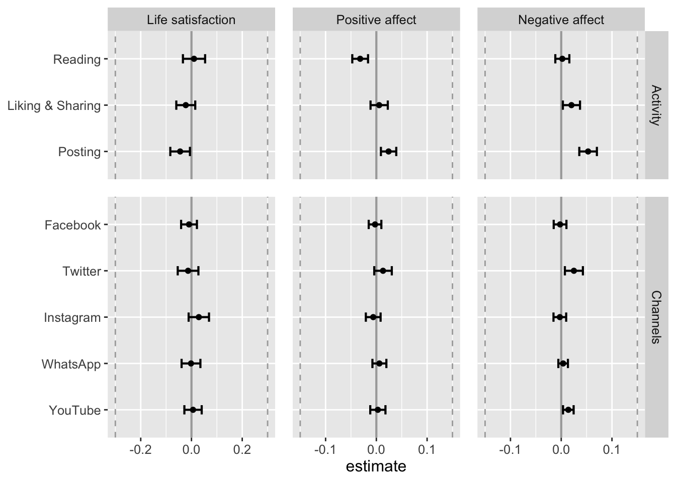

# save figure
ggsave("figures/fig_results_within.png", 
       width = 7, height = 4,
       plot = fig_results_within)

Let’s next visualize standardized predictors, to allow for better comparison across differently scaled variables.

# make figure
data_tab_comp_std <- rbind(
  get_dat_res(fit_aff_neg_lmer_std, fit_aff_pos_lmer_std, fit_life_sat_lmer_std, 
              type = "Activity", variance = "within", analysis = "standardized"),
  get_dat_res(fit_aff_neg_lmer_std, fit_aff_pos_lmer_std, fit_life_sat_lmer_std, 
              type = "Channels", variance = "within", analysis = "standardized"),
  get_dat_res(fit_aff_neg_lmer_std, fit_aff_pos_lmer_std, fit_life_sat_lmer_std, 
              type = "News\nuse", variance = "within", analysis = "standardized"),
  get_dat_res(fit_aff_neg_lmer_std, fit_aff_pos_lmer_std, fit_life_sat_lmer_std, 
              type = "Living\nconditions", variance = "within", analysis = "standardized"),
  get_dat_res(fit_aff_neg_lmer_std, fit_aff_pos_lmer_std, fit_life_sat_lmer_std, 
              type = "Outdoor\nactivities", variance = "within", analysis = "standardized"),
  get_dat_res(fit_aff_neg_lmer_std, fit_aff_pos_lmer_std, fit_life_sat_lmer_std, 
              type = "Psycho-\nlogy", variance = "within", analysis = "standardized")
  )

fig_results_comp_std <- make_graph_res(
  data = data_tab_comp_std,
  sesoi = "std",
  legend = FALSE
  , facet = "type"
  # , title = "Results of selected covariates"
  )
fig_results_comp_std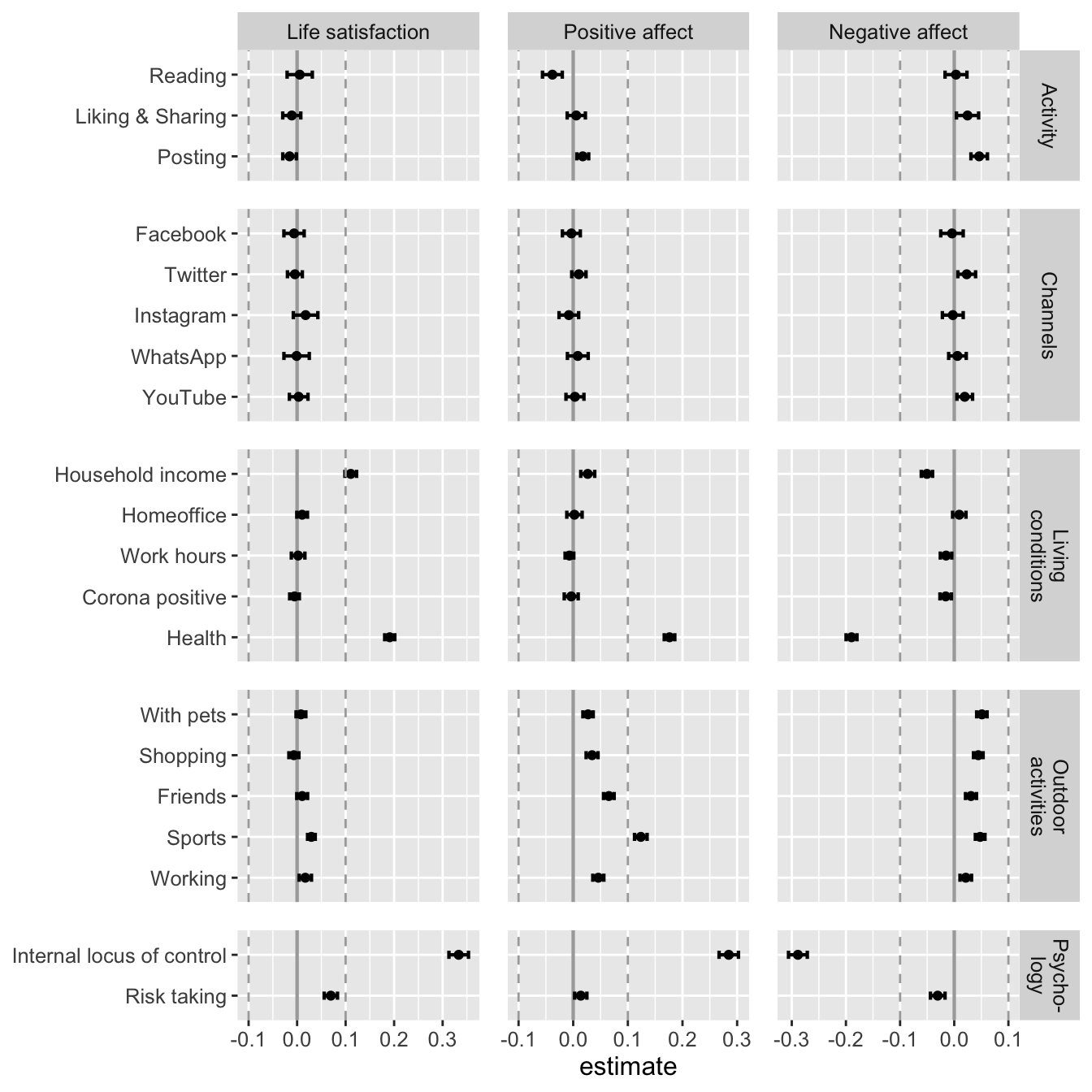

# save figure
ggsave("figures/fig_results_comp_std.png", 
       width = 7, height = 7,
       plot = fig_results_comp_std)

Table

Let’s extract results for a table of within-person effects.

tab_within <-
  data_tab_comp_std %>% 
  filter(Type %in% c("Activity", "Channels")) %>% 
  select(std = estimate) %>% 
  cbind(data_tab_within) %>% 
  mutate(p.value = td::my_round(p.value, "p")) %>% 
  arrange(dv) %>% 
  select(Outcome = dv,
         Predictor = iv,
         b = estimate,
         `Lower` = conf.low,
         `Higher` = conf.high,
         beta = "std",
         p = "p.value")

tab_within

ABCDEFGHIJ0123456789

Outcome <fct>	Predictor <fct>	b <dbl>	Lower <dbl>	Higher <dbl>	beta <dbl>	p <chr>
Life satisfaction	Reading	0.0100	-0.0337	0.0537	0.0054	.639
Life satisfaction	Liking & Sharing	-0.0225	-0.0598	0.0149	-0.0110	.227
Life satisfaction	Posting	-0.0447	-0.0834	-0.0060	-0.0155	.025
Life satisfaction	Facebook	-0.0097	-0.0408	0.0215	-0.0063	.527
Life satisfaction	Instagram	0.0290	-0.0112	0.0691	0.0175	.149
Life satisfaction	WhatsApp	-0.0019	-0.0389	0.0352	-0.0010	.917
Life satisfaction	YouTube	0.0062	-0.0280	0.0403	0.0032	.713
Life satisfaction	Twitter	-0.0135	-0.0542	0.0273	-0.0045	.503
Positive affect	Reading	-0.0319	-0.0474	-0.0164	-0.0381	< .001
Positive affect	Liking & Sharing	0.0055	-0.0115	0.0225	0.0056	.508
Positive affect	Posting	0.0241	0.0090	0.0392	0.0175	.003
Positive affect	Facebook	-0.0026	-0.0150	0.0098	-0.0034	.671
Positive affect	Instagram	-0.0062	-0.0207	0.0084	-0.0080	.390
Positive affect	WhatsApp	0.0060	-0.0077	0.0197	0.0084	.374
Positive affect	YouTube	0.0030	-0.0120	0.0179	0.0032	.686
Positive affect	Twitter	0.0131	-0.0041	0.0304	0.0104	.130
Negative affect	Reading	0.0022	-0.0116	0.0160	0.0032	.747
Negative affect	Liking & Sharing	0.0201	0.0032	0.0370	0.0246	.022
Negative affect	Posting	0.0530	0.0356	0.0703	0.0461	< .001
Negative affect	Facebook	-0.0023	-0.0148	0.0103	-0.0042	.710

Save workspace

First remove large objects

rm(fig_cor)

save.image("data/workspace_2.RData")

Beyens, Ine, J. Loes Pouwels, Irene Ingeborg van Driel, Loes Keijsers, and Patti M. Valkenburg. 2021. “Social Media Use and Adolescents’ Well-Being: Developing a Typology of Person-Specific Effect Patterns.” Communication Research. https://doi.org/10.1177/00936502211038196.

Funder, David C., and Daniel J. Ozer. 2019. “Evaluating Effect Size in Psychological Research: Sense and Nonsense.” Advances in Methods and Practices in Psychological Science 2 (2): 156–68. https://doi.org/10.1177/2515245919847202.

wave <dbl>	value <dbl>
1	1.4
2	1.4
3	1.4
4	1.4
5	1.4
6	1.4
7	1.4
8	1.4
9	1.4
10	1.4
11	1.4
12	1.4
13	1.4
14	1.4
15	1.4
16	1.4
17	1.4
18	1.4
19	1.4
20	1.4

wave <dbl>	value <dbl>
1	1.4
2	1.4
3	1.4
4	1.4
5	1.4
6	1.4
7	1.4
8	1.4
9	1.4
10	1.4
11	1.4
12	1.4
13	1.4
14	1.4
15	1.4
16	1.4
17	1.4
18	1.4
19	1.4
20	1.4

wave <dbl>	value <dbl>
1	1.4
2	1.4
3	1.4
4	1.4
5	1.4
6	1.4
7	1.4
8	1.4
9	1.4
10	1.4
11	1.4
12	1.4
13	1.4
14	1.4
15	1.4
16	1.4
17	1.4
18	1.4
19	1.4
20	1.4